
Create successful ePaper yourself
Turn your PDF publications into a flip-book with our unique Google optimized e-Paper software.
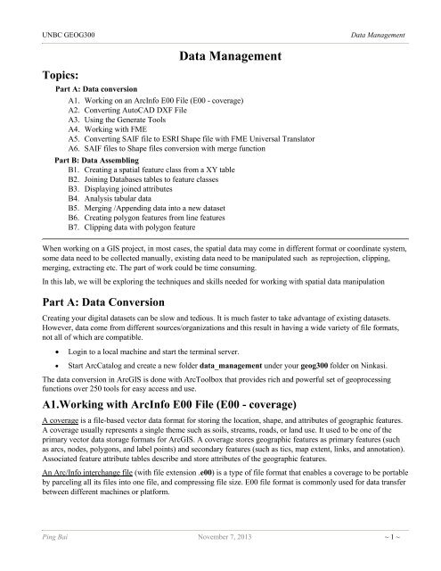
<strong>UNBC</strong> GEOG300<br />
<strong>Data</strong> <strong>Management</strong><br />
Topics:<br />
Part A: <strong>Data</strong> conversion<br />
<strong>Data</strong> <strong>Management</strong><br />
A1. Working on an ArcInfo E00 File (E00 - coverage)<br />
A2. Converting AutoCAD DXF File<br />
A3. Using the Generate Tools<br />
A4. Working with FME<br />
A5. Converting SAIF file to ESRI Shape file with FME Universal Translator<br />
A6. SAIF files to Shape files conversion with merge function<br />
Part B: <strong>Data</strong> Assembling<br />
B1. Creating a spatial feature class from a XY table<br />
B2. Joining <strong>Data</strong>bases tables to feature classes<br />
B3. Displaying joined attributes<br />
B4. Analysis tabular data<br />
B5. Merging /Appending data into a new dataset<br />
B6. Creating polygon features from line features<br />
B7. Clipping data with polygon feature<br />
When working on a <strong>GIS</strong> project, in most cases, the spatial data may come in different format or coordinate system,<br />
some data need to be collected manually, existing data need to be manipulated such as reprojection, clipping,<br />
merging, extracting etc. The part of work could be time consuming.<br />
In this lab, we will be exploring the techniques and skills needed for working with spatial data manipulation<br />
Part A: <strong>Data</strong> Conversion<br />
Creating your digital datasets can be slow and tedious. It is much faster to take advantage of existing datasets.<br />
However, data come from different sources/organizations and this result in having a wide variety of file formats,<br />
not all of which are compatible.<br />
<br />
<br />
Login to a local machine and start the terminal server.<br />
Start ArcCatalog and create a new folder data_management under your geog300 folder on Ninkasi.<br />
The data conversion in Arc<strong>GIS</strong> is done with ArcToolbox that provides rich and powerful set of geoprocessing<br />
functions over 250 tools for easy access and use.<br />
A1.Working with ArcInfo E00 File (E00 - coverage)<br />
A coverage is a file-based vector data format for storing the location, shape, and attributes of geographic features.<br />
A coverage usually represents a single theme such as soils, streams, roads, or land use. It used to be one of the<br />
primary vector data storage formats for Arc<strong>GIS</strong>. A coverage stores geographic features as primary features (such<br />
as arcs, nodes, polygons, and label points) and secondary features (such as tics, map extent, links, and annotation).<br />
Associated feature attribute tables describe and store attributes of the geographic features.<br />
An Arc/Info interchange file (with file extension .e00) is a type of file format that enables a coverage to be portable<br />
by parceling all its files into one file, and compressing file size. E00 file format is commonly used for data transfer<br />
between different machines or platform.<br />
Ping Bai November 7, 2013 ~ 1 ~
<strong>UNBC</strong> GEOG300<br />
<strong>Data</strong> <strong>Management</strong><br />
Import an E00 file to ArcInfo Coverage<br />
The E00 file we are going to convert to coverage is lakes.e00 located at N:\labs\geog300\conversion<br />
As an E00 file is not a spatial data format, you can't see them in the catalog tree in ArcCatalog by default. If you<br />
want to see them, you have to add the file type to the ArcCatalog.<br />
<br />
<br />
<br />
In ArcCatalog. Click the Customize->ArcCatalog Option and click File Types tab. Here you can add more<br />
file types to allow them to be listed in the catalog tree.<br />
Click New Type button. In the popped up window, give E00 for the file extension and 'ArcInfo Interexchange<br />
file' for the Description and click OK button.<br />
Back to ArcCatalog and navigate to N:\labs\geog300\conversion, you should be able to find the file<br />
lakes.e00.<br />
The conversion can be done in either ArcCatalog or ArcMap. Click the toolbox button to open it<br />
<br />
<br />
<br />
<br />
<br />
<br />
<br />
In ArcToolbox, click Coverage Tools->Conversion->To Coverage.<br />
Double-click Import from Interchange File. A small window pops up asking for input file and output<br />
dataset.<br />
Leave the Feature Type as it is.<br />
Set N:\labs\geog300\conversion\lakes.e00 to Input File OR you can click on the Open folder button to<br />
browse the directory.<br />
Set N:\username\geog300\data_management\lakes to Output <strong>Data</strong>set or click the Open folder and<br />
navigate to your data_management directory and give the dataset name to lakes. Note: the username<br />
should be replaced by your user account.<br />
Click OK to run the conversion.<br />
Examine the lakes in your local folder<br />
Export ArcInfo coverage to E00 file<br />
Similarly you can export ArcInfo coverage to an E00 file for transferring purposes. When exporting a coverage, all<br />
associated INFO tables will be written to the interchange file.<br />
<br />
<br />
<br />
<br />
<br />
In ArcToolbox, click Coverage Tools->Conversion->From Coverage->Export to Interchange File.<br />
Set N:\username\geog300\data_management\lakes (your local copy) to Input <strong>Data</strong><br />
Set N:\username\geog300\data_management\lakes_export.e00 to Output<br />
Click OK to run the conversion.<br />
Once done, you should have an E00 file lakes_export.e00 listed under your data_management folder.<br />
Convert a coverage to shape file<br />
A coverage can be easily saved in shape file format if needed<br />
<br />
<br />
<br />
In ArcCatalog, navigate to your local folder N:\username\geog300\data_management<br />
Look at the dataset lakes you just converted from E00 file. Click the plus sign beside lakes.<br />
Right-click on Polygon under lakes and choose Export->To Shape Single. Save it as lakes_shape.shp in<br />
your local folder.<br />
Ping Bai November 7, 2013 ~ 2 ~
<strong>UNBC</strong> GEOG300<br />
<strong>Data</strong> <strong>Management</strong><br />
A2. Import AutoCAD DXF File<br />
AutoCAD, drafting software, has been on the market for a login time. Taking advantage of the digital version of<br />
spatial data in AutoCAD format will be a time saver. A DXF file is an AutoCAD Drawing Interchange File and<br />
can be converted to either Shpaefile or ArcInfo coverage format.<br />
Convert DXF file to shapefile format<br />
The DXF file we will be working is creeks.dxf located at N:\labs\geog300\conversion<br />
Click Conversion Tools->To Shapefile->Feature Class to Shapefile<br />
Click the open folder button for the Input Feature and navigate to N:\labs\geog300\conversion\. Double<br />
creek.dxf and click Polyline. Click OK. This will convert only line feature.<br />
Set N:\username\geog300\data_management for the Output folder, or click the Open folder and navigate<br />
to your data_management directory. Click OK to run the conversion.<br />
Preview the creeks in ArcCatalog.<br />
A3. Using the Generate Tools<br />
Spatial location information can be saved in a text file. The text file contains x,y coordinates for points, lines and<br />
polygon. In this part of the lab, you will be working with the ArcInfo Generate tool to create spatial data from text<br />
files.<br />
The Generate tool allows you to create spatial data from a text file or from the input entered by the user.<br />
The text file used for this conversion is greenway.txt located at N:\labs\geog300\conversion\<br />
Take a look at the greenway.txt file.<br />
<br />
<br />
Click Start->Accessories-> Notepad to open a text editor.<br />
Click File->Open and navigate to N:\labs\geog300\conversion. Click<br />
greenway.txt to open the file. You should see that the content of the text file<br />
looks like the picture showing at right.<br />
The numbers 1 and 2 separated from the rest indicate the sections code for different<br />
line segments. Each whole number indicates a beginning of a line feature and END<br />
indicates the end of a line feature. A pair of numbers separated by a comma<br />
(510239.83, 5970539.44) is the coordinates of a vertex along the line feature.<br />
<br />
<br />
<br />
<br />
<br />
<br />
Close NotePad<br />
In the ArcToolbox, click Coverage Tools->Conversion->To Coverage->Generate<br />
Set the Input File to N:\labs\geog300\conversion\greenway.txt<br />
Set N:\username\geog300\data_managemet\greenway for the<br />
Output Coverage<br />
Choose LINES for Feature Type and click OK.<br />
Once done, you should see greenway in your<br />
data_management folder. Examine the data.<br />
1<br />
511520.78, 5969179.67<br />
511535.70, 5969200.48<br />
511540.53, 5969236.94<br />
511547.72, 5969268.34<br />
511567.78, 5969296.34<br />
511586.55, 5969310.14<br />
511617.02, 5969328.88<br />
END<br />
2<br />
510239.83, 5970539.44<br />
510221.73, 5970497.97<br />
510194.81, 5970414.39<br />
510185.30, 5970386.56<br />
.......<br />
Although the Generate Tool can generate a spatial data from a text file,<br />
it can't carry any non spatial data with it. If you need non-spatial information for each spatial feature, you need to<br />
add or join attributes to the feature attribute table afterwards for symbolization or analysis.<br />
Ping Bai November 7, 2013 ~ 3 ~
<strong>UNBC</strong> GEOG300<br />
<strong>Data</strong> <strong>Management</strong><br />
A4. Working with FME - Converting SAIF file to Shape file<br />
We have examined the way of converting spatial data from one format to another in Arc<strong>GIS</strong>. But there are some<br />
limitations with Arc<strong>GIS</strong> conversion tools. Some third party software provides more powerful tools for data<br />
conversion in many different formats.<br />
FME (Feature Manipulation Engine) is a powerful software tool that can extract, transform and load spatial data.<br />
This software is capable of doing these operations with many different file formats. FME consists of three main<br />
components: Universal Translator which works basically in batch mode on translation, Workbench, a GUI<br />
interface allowing interactively customize the translation, and Universal Viewer, a Viewer to examine the spatial<br />
data<br />
In this part of lab you will be exploring useful tools in FME software.<br />
The spatial data we will be working on are in SAIF format (pronounced safe), Spatial Archive and Interchange<br />
Format, is a Canadian geomatics standard for the exchange of geographic data. BC TRIM data (Terrain Resource<br />
Information <strong>Management</strong>) are in SAIF format.<br />
We will first examine a SAIF file in the FME Viewer.<br />
<br />
<br />
Click Start->FME Suite->FME Universal Viewer to open the FME Viewer.<br />
Click File->Open <strong>Data</strong>set and navigate to N:\labs\geog300\conversion\. Click 82m019.saf to open it.<br />
You probably notice that many TRIM layers are listed in the table of contents. Examine each layer.<br />
<br />
<br />
<br />
<br />
<br />
<br />
<br />
Now start FME Universal Translator. Click Start->All Programs->FME ->FME Universal Translator<br />
Click Translate <strong>Data</strong> button (the first button) on the menu bar to specify parameters.<br />
Set the parameters like the image right above.<br />
Set Destination <strong>Data</strong>set to N:\username\geog300\data_management\trim. Note: The Destination<br />
<strong>Data</strong>set should be your local folder.<br />
In the popped up window, choose ‘updated’ for Version and<br />
‘full_attribution’ for Attribute Type<br />
Click OK to run the translation. All output layers will be saved<br />
under trim folder<br />
In ArcCatalog, examine your data_management/trim folder.<br />
You will get the following layers:<br />
Ping Bai November 7, 2013 ~ 4 ~
<strong>UNBC</strong> GEOG300<br />
<strong>Data</strong> <strong>Management</strong><br />
Layers Description Layers Description<br />
tctrl Contours trivr Rivers<br />
tcull Cultural feature lines troad Roads<br />
tculp Cultural feature points tsymb Symbol locations<br />
tcvrl Land Cover ttext Annotations<br />
tspht Spot height ttrnl Transportation<br />
tsfl Surface line features twtrl Water feature lines<br />
tlake Lakes twtrp Water feature points<br />
Examine tctrl.shp (the contour lines), what is the elevation interval?<br />
Examine tlake.shp (lakes), how many definite and Intermittent lakes respectively (TYPE)?<br />
Examine troad.shp (roads)), are there any "Paved Road 2 Lane" roads? If yes, how many?<br />
A5. SAIF to Shape files conversion in FME with merging function<br />
In general, spatial data are stored based on mapsheet which is defined by standard mapping grid such as NTS,<br />
BCNTS etc. In some cases, your study/working area maybe quite large and require more than one mapsheet to<br />
cover the area. In this case, you can do the conversion and the data merging in one step with FME<br />
Assume that our study area is Fraser River Park located south of Prince George. The Fraser River Park is covered<br />
by three 1:20k map sheets. The mapsheet numbers are: 093G047, 093G056 and 093G057. We want to convert<br />
them to shapefiles and merge all required layers from all sheets together at the same time.<br />
<br />
<br />
Start FME Translator<br />
Set the Spatial Archive and Interchange Format (SAIF) for Source Format<br />
Click the Browse button and navigate to N:\labs\goeg300\conversions\ folder. Hold Ctrl and click<br />
93g047.saf, 93g056.saf and 93g057.saf to add them all as Source dataset.<br />
<br />
<br />
<br />
<br />
<br />
<br />
<br />
Make sure the radio button beside 'Merge source datasets to one destination' is checked. This will result in<br />
layers from each map sheet being merged together based on the feature type.<br />
Set the Destination Format to ESRI Shape and Destination<br />
<strong>Data</strong>set to<br />
N:\username\geog300\data_management\trim_merge<br />
Choose BC TRIM II (after03/01/00) in SAIF to Shape<br />
Translation and click OK.<br />
Set Updated for Version and full_attribution for Attribute<br />
Type in the popped up window. Click OK.<br />
Once the conversion is done, you should have all spatial<br />
layers for the area of Fraser River Park in your<br />
trim_merge folder.<br />
Open an empty map file in ArcMap. Add the Fraser River<br />
Park boundary fraser_river_park from<br />
N:\labs\geog300\fraser_river_park folder. Add traod,<br />
trivr, tlake and tctrl from your local folder<br />
Examine the datasets.<br />
Ping Bai November 7, 2013 ~ 5 ~
<strong>UNBC</strong> GEOG300<br />
<strong>Data</strong> <strong>Management</strong><br />
Fraser River Park boundary with 1:20k map<br />
sheets<br />
Fraser River Park boundary with data from<br />
093G047, 056, 057<br />
Part B: <strong>Data</strong> Assembling<br />
We have done data conversion job in the previous steps. In this part of lab we will go through some basic steps for<br />
spatial data manipulation such as working with CSV file and tabular data, projections, spatial data appending,<br />
clipping etc.<br />
B1. Creating a spatial feature class from a CSV file<br />
Arc<strong>GIS</strong> allows you to work with attribute tables and CSV file (Comma Separated Values). We have two files<br />
plots.xls and plots_attr.xls containing sampling plot locations and their attributes respectively in Excel format.<br />
plots.xls contains sampling plot locations with three columns plot_id, x_coord, y_coord separated by commas.<br />
plot_id is the plot id for each spatial location, x_coord contains X coordinate and y_coord is the y coordinate for<br />
each location. plots_attr.xls contains the attributes of each sampling plot in plots.xls<br />
<br />
<br />
<br />
<br />
<br />
<br />
<br />
<br />
<br />
<br />
In ArcCatalog, navigate to N:\labs\geog300\unbc. Click the plus sign beside plots.xls to show the conents.<br />
Highlight plots$ to preview the data. It contains the plot locations<br />
Right-click plots$ and choose Create Feature Class->From XY table.<br />
Choose x_coord for X Field and y_coord for Y Field.<br />
Click the ‘Coordinate System of Input Coordinates’ button. Here you can specify the coordinate system.<br />
As the xy coordinates are in UTM 10 projection so we should specify UTM 10.<br />
Click Projected Coordinate System->UTM->NAD 1983->NAD1983 UTM Zone 10N. Click OK.<br />
Set the Output to N:\username\geog300\data_managament\plots.shp<br />
Click OK to generate the shape file plots.shp. You will have a point feature dataset created in your local<br />
folder. Examine plots.shp<br />
Now export the attribute of plots to a dBase table. Back to N:\labs\geog300\unbc folder and expand<br />
plots_attr.xls. Right-click plots_attr$ and choose Export->to dBase single<br />
Set the output location to N:\username\geog300\data_management<br />
Set plots_attr.dbf to Output Table and click OK. A dbase version of plots_attr.dbf is listed under your<br />
local folder<br />
Ping Bai November 7, 2013 ~ 6 ~
<strong>UNBC</strong> GEOG300<br />
<strong>Data</strong> <strong>Management</strong><br />
B2. Joining tables to feature classes<br />
Sometimes the data you want to use for display/analysis are not physically stored together with spatial data. They<br />
are stored in a separate file/table. Usually this type of information is called non-spatial data. The non-spatial<br />
information has to be associated to the spatial feature by joining the table to the spatial data for data display, query<br />
and analysis.<br />
Typically, you'll join a table of data to a layer based on the value of a field that can be found in both tables. The<br />
name of the field does not have to be the same name, but the data type of both fields has to be the same. JOIN<br />
operation combines records from two tables, resulting in a new, temporary table, sometimes called a "joined table"<br />
or virtual join. You may also think of JOIN as an operation that relates tables of values common between them.<br />
We have a point feature class plots.shp created from the XY table in the previous section, which contains the<br />
locations of plots. We have a DBF file plots_attr.dbf containing the attribute information of the sampling plots.<br />
We want to join the attribute table plots_attr.dbf to the plots feature table so that we can query the non-spatial<br />
data, such as stand age, height classes, leading species etc. stored in plots_attr.dbf. These two tables are in a one<br />
to one relationship.<br />
plots table<br />
Now minimize ArcCatalog window.<br />
<br />
<br />
Start ArcMap with a new empty map file.<br />
plots_attr.dbf<br />
Add dataset plots.shp and plots_attr.dbf table from your geog300\data_management folder.<br />
The plots is a point feature class while the plots_attr.dbf is a table containing the descriptions of each sampling<br />
plot. You probably wouldn't see plots_attr.dbf from the table of contents in Display mode as it is not spatial data.<br />
You need to switch to Source mode in the table of contents (check the tabs located at lower left corner)<br />
Look at the button at the top in the table of contents. The buttons allow you to display data layers in different way.<br />
o The first button from left: List layers by Drawing order<br />
o The second button from left: List layers by Source<br />
o The third button from left: List layers by Visibility<br />
o The fourth button from left: List layers by Selection<br />
<br />
<br />
<br />
Click the second button (List by Source). The plots_attr.dbf is listed there.<br />
Back to Display mode by clicking the first button (List by Drawing order).<br />
Examine the attribute of plots.shp. There is no any description for each spatial feature<br />
A relationship between two tables is maintained through attribute values for key fields. To join two tables, a<br />
primary key and foreign key are needed as a common join item. The primary key is a field in a table which is<br />
uniquely identifies each record. The foreign key is a data field in one table and the primary key in the second table.<br />
This data field usually is used for linking the two tables.<br />
Ping Bai November 7, 2013 ~ 7 ~
<strong>UNBC</strong> GEOG300<br />
<strong>Data</strong> <strong>Management</strong><br />
In our case, we will use plot_id from both tables as a join item to<br />
perform the Join operation.<br />
<br />
<br />
<br />
<br />
<br />
<br />
Right-click on the plots layer in the table of contents and<br />
choose Join and Relate->Join<br />
Set 'Join Attribute to Table' to 'What do want to join to<br />
this layer'<br />
Click dropdown list for #1 'Chose the field in this layer<br />
that the join will be based on'. Choose PLOT_ID. This<br />
defines the data field used for Join in the first table (plots).<br />
Click the dropdown list for #2 'Choose the table to join to<br />
this layer or Load the table from disk'. Choose<br />
plots_attr.dbf. This specifies the table you want to join<br />
the first table.<br />
Set the join item to PLOT_ID for #3 'Choose the field in the table to base the join on'. This defines the join<br />
item from the second table (plots_attr.dbf). Click OK.<br />
Now right-click plots layer and choose Open Attribute Table. You should see the attributes from table<br />
plots_attr.dbf are appended into the plots.php feature attribute table. These attributes can be used later for<br />
querying and analysis purpose.<br />
Note that the plotts_attr.dbf table is not physically appended to the end of the plots.shp attribute table. It is a<br />
virtual join.<br />
If you want keep everything in one dataset, you can export plots.shp to a new dataset with all joined attributes<br />
To export plots.shp, right-click on plots.shp-><strong>Data</strong>-><strong>Data</strong> Export. Go to your local folder and save it<br />
plots_export.shp. When prompt to add data to ArcMp, click No to not add it into ArcMap<br />
B3. Displaying joined attributes<br />
Attributes joined into spatial feature can be displayed, queried and analyzed.<br />
Now display the plots layer using stand age<br />
<br />
<br />
<br />
<br />
Right-click plots layer and choose Properties. Click on Symbology<br />
tab.<br />
Click on Quantities and choose Graduated Symbol. Set stand_age to<br />
Value Field and take the default number of classification (5 classes)<br />
Click OK. This will display the layer based on the range of stand<br />
age. The bigger circle represent the older ages.<br />
Now display plots using the leading species (sp1) and height classes<br />
(height_cl) respectively.<br />
You can also query the data with the joined information. For example, we want to know how many are SPRUCE<br />
plots (sp1: S) and how many plots fall into the range 100 to 130 on stand age.<br />
Ping Bai November 7, 2013 ~ 8 ~
<strong>UNBC</strong> GEOG300<br />
<strong>Data</strong> <strong>Management</strong><br />
<br />
<br />
<br />
First find out the number of plots that have SPRUCE as the leading species, click Selection ->Select by<br />
Attributes<br />
ArcMap list all data fields in the attribute table here. Click SP1 from the field list and click Get Unique<br />
Values button. Arc<strong>GIS</strong> lists all unique values from SP1 field.<br />
Double click SP1 from the field list and click the equal sign button and double click 'S' from the value<br />
list to build up a query expression.<br />
"SP1" = 'S'<br />
<br />
<br />
Click OK to run the query. All the plots with spruce as their leading species are highlighted in cyan color.<br />
Check the display and the attribute table. The total number of selected features can be found at the bottom<br />
of attribute table.<br />
Follow the same steps to find the plots falling into range 100 to 130 on stand age. Here is the query<br />
expression should look like:<br />
"STAND_AGE" > 100 AND "STAND_AGE" < 130<br />
<br />
Save your map file to management.mxd under your data_management folder.<br />
What is the total number of spruce plots?<br />
How many plots fall into the range 100 to 130 on stand age?<br />
<br />
Now clear the selection by right-click plots and choose Selection->Clear Selection.<br />
B4. Analysis of tabular data<br />
Analyzing tabular data often involves finding how many of features belong to a given category, or looking at the<br />
distribution of values for a set of features.<br />
Finding how many<br />
Sometimes we want to analyze the information in the attribute table such as finding the sum of some field for<br />
selected features, or the frequency of a particular feature type. The Summary Statistics and Frequency tools allow<br />
you to calculate these statistics on a field or several fields, and to summarize the results accordingly. This can be<br />
useful for reporting as well as analysis.<br />
Now find out what the average stand age is on all plots.<br />
<br />
Open the attribute table of plots. Right-click on stand_age field and choose Statistics<br />
Here you can find all statistic information on stand_age such as average, min, max etc.<br />
What is the average, min and max values on stand height (stand_ht) for all features respectively?<br />
Ping Bai November 7, 2013 ~ 9 ~
<strong>UNBC</strong> GEOG300<br />
<strong>Data</strong> <strong>Management</strong><br />
Sometimes we want some information on the features that meet specific criteria. For example, the average stand<br />
height (stand_ht) for all Douglas Fir ("FD" in sp1) plots.<br />
<br />
<br />
<br />
<br />
<br />
First we need to find all Douglas Fir plots by applying an attribute based query. Click Selection->Select by<br />
Attributes from the top menu<br />
In the query builder, build a query with following expression (as you did in previous section) and click OK<br />
"SP1" = 'FD'<br />
Open the attribute table and click the toggle button<br />
‘Show Selected’ located at the bottom of the table to show the only selected features.<br />
Now right-click stand_ht and choose Statistics. Here you can find average stand height for only Douglas<br />
Fir plots.<br />
What is the average, min and max values on stand height (stand_ht) for Douglas Fir plots<br />
respectively?<br />
Clear the selection<br />
Calculating frequency with the Frequency tool is a good way to learn how many of features fall into a given<br />
category. For example, you might run the tool on a set of parcels to see how many belong to each of several land<br />
use categories. Looking at the frequency distribution of your categorical data is an important first step in many<br />
analyses.<br />
Now examine the leading species to see what the total number of plots have which leading species<br />
<br />
<br />
<br />
<br />
Right-click on sp1 (leading species) and choose Summarize. Set the output table to<br />
N:\username\geog300\data_managament\sum_sp1 and take the default for everything else<br />
Click OK. You will have a table sum_sp1.dbf saved in your management folder.<br />
Click Yes when prompted if you want to add the table to ArcMap. You will have<br />
this table showing in ArcMap.<br />
Right-click on sum_sp1.dbf and choose Open to open the table.<br />
This frequency table tells you the total number of plots (Count_sp1) for each leading<br />
species. You can tell from the table, the smallest number of plots has the leading species<br />
'SB'.<br />
Calculating Field values<br />
The Field Calculator tool is used to mathematically combine or manipulate values in one or more fields. These<br />
calculations can be as simple as calculating a given field to "23" for all features, or to "true" for all selected<br />
features, or to combine values in multiple fields. For example, you might divide a population field by an area field<br />
to get population density values, or concatenate the text from house number, street name, and street type fields into<br />
a single address field. Many times, you want to add a new field using the Add Field tool to contain the results of<br />
your calculation.<br />
<br />
<br />
<br />
In ArcCatalog, copy the dataset ea96_den_kids.shp from N:\labs\geog300\pgcity to your<br />
data_management folder.<br />
Add your local copy of ea96_den_kids.shp into ArcMap.<br />
Open the attribute table to examine attributes. The field pop96 contains the population of each EA polygon<br />
and the area_skm have the area of each polygon in square kilometres.<br />
Ping Bai November 7, 2013 ~ 10 ~
<strong>UNBC</strong> GEOG300<br />
<strong>Data</strong> <strong>Management</strong><br />
Assume that each dwelling has average two kids at school age. The total number of kid at school age can be used<br />
as a factor to determine if there is a need for such as a new elementary school etc. We need to add the data fields<br />
DENSITY and SCH_KIDS to the table and then assign the calculated values to these fields.<br />
<br />
<br />
<br />
<br />
<br />
Now add DENSITY and SCH_KIDS fields using the specification<br />
listed at right<br />
Now we can assign values to these fields. Right-click on the field<br />
DENSITY and choose Field Calculator. Here you can build<br />
expression to assign values to the field.<br />
Double click the field POP96 from the field list and type in / and double click AREA_SM to make up a<br />
expression<br />
[POP96] / [AREA_SKM]<br />
Click OK. The calculated values will be assigned to the data field DENSITY to indicate the density of<br />
population.<br />
Calculate field SCH_KIDS with the following expression in the same way (assume that each family has<br />
two children at school age)<br />
[DEWELL96] * 2<br />
DENSITY SCH_KIDS<br />
Type Double Sort Integer<br />
Precision 10 5<br />
Scale 1 0<br />
<br />
<br />
Now use the DENSITY field and SCH_KIDS to display the data respectively (symbology)<br />
Save the map file in your local folder<br />
What is the population density of the largest polygon?<br />
What is the total number of kids at school age for entire Prince George?<br />
B5. Merging/Appending data<br />
Spatial data are often stored based on the map sheets such as 1:250,000 sheets, 1:50,000 sheets (NTS) and 1:20,000<br />
sheets (TRIM) etc. In some cases, you need more than one map sheet to cover your study area. In this case, you<br />
will need to merge the data from two or more map sheets together for your study area.<br />
We have examined how we can use FME to do the merging task. In some cases, we may need to do this manually<br />
due to spatial data from difference sources and format. Here we will explore techniques in Arc<strong>GIS</strong> for data<br />
manipulating<br />
Digital Terrain Resource Information <strong>Management</strong> (TRIM) topographic database is at 1:20 000 scale for the<br />
Province of BC. A number of spatial themes are included such as contours, water bodies and roads and railways.<br />
Minimal attribute data is available. TRIM data contains enhanced road and hydrographic networks and additional<br />
land cover features such as cut blocks and log landings.<br />
The study area is Fraser River Park located to the south of Prince George. Three TRIM sheets are needed to cover<br />
the park's boundary (093g047, 093g056 and 093g057). There are many data layers in each map sheet. We only<br />
need contours, lakes, rivers and roads layers. The layer name and the description are listed in the table at below<br />
<br />
Now back to ArcMap, open a new empty file and add the following datasets<br />
from N:\labs\geog300\fraser_river_park<br />
93g047_tctrl, 93g047_tlake, 93g047_trivr, 93g047_troad,<br />
93g056_tctrl, 93g056_tlake, 93g056_trivr, 93g056_troad,<br />
93g057_tctrl, 93g057_tlake, 93g057_trivr, 93g057_troad<br />
TRIM layers Description<br />
tctrl Contours<br />
tlake Lakes<br />
trivr Rivers<br />
troad Roads<br />
We will merge contours, lakes, rivers and roads from each sheet to make a new dataset respectively.<br />
Ping Bai November 7, 2013 ~ 11 ~
<strong>UNBC</strong> GEOG300<br />
<strong>Data</strong> <strong>Management</strong><br />
<br />
Turn on the ArcToolbox by clicking the toolbox if necessary.<br />
In ArcToolbox, click <strong>Data</strong> <strong>Management</strong> Tools->General->Merge<br />
Click the dropdown arrow for Input <strong>Data</strong>set and choose 93g047_tctrl, 93g056_tctrl, 93g057_tctrl (all<br />
contours)<br />
Set the output dataset to N:\username\geog300\data_managament\contours_merge and click OK.<br />
A new dataset will be created with three data sheets merged together. Once it is done, the new dataset<br />
contours_merge will be added to ArcMap.<br />
<br />
<br />
Now following the same steps to merge lakes, rivers and roads respectively. Give the name lakes_merge,<br />
rivers_merge, roads_merge respectively for the output in your local folder.<br />
Once done, remove the following original layers by right-click on the layer and choose Remove.<br />
93g047_tctrl, 93g047_tlake, 93g047_trivr, 93g047_troad,<br />
93g056_tctrl, 93g056_tlake, 93g056_trivr, 93g056_troad,<br />
93g057_tctrl, 93g057_tlake, 93g057_trivr, 93g057_troad<br />
B6. Creating polygon features from line features<br />
Examine the dataset lakes_merge, you may notice that the lakes_merge is a line feature. It should be in closed<br />
polygon features in this case. This is because all TRIM data come in either point features or line features. The<br />
polygon features have to be created from the line features if necessary.<br />
We will build up a polygon feature class from the lake outline. This can be done with Feature to Polygon tool in<br />
ArcToolbox.<br />
<br />
<br />
<br />
<br />
<br />
<br />
<br />
<br />
<br />
<br />
<br />
Leave lakes_merge on and turn off the rest of layers.<br />
Open the attribute table of lakes_merge check the data field CLASS. The information in this field tells you<br />
the feature class.<br />
Sort the CLASS field by right-click on CLASS field and choose Ascending or Descending. You may<br />
notice that some of features are type of Lake and some of them are Reservoir. We need to extract all the<br />
Lake features<br />
Make a query with Select by Attribute to pull out all Lake with following query expression<br />
"CLASS" = 'Lake'<br />
Now you have a selection for Lakes.<br />
With this selection on, in the ArcToolbox, click<br />
<strong>Data</strong> <strong>Management</strong> Tool->Features->Feature to Polygon<br />
In the dialog window, click the dropdown list for Input Features and choose lakes_merge<br />
Click the button right to the Output Feature Class and navigate to your local folder data_management and<br />
give the name lakes_poly for the output dataset<br />
Click OK. Once finished, the new dataset lakes_poly with polygon features will be added to ArcMap.<br />
Examine lakes_merge and lakes_poly. You probably notice that some lake lines from lakes_merge do not<br />
show in lakes_poly. This is because we have a selection on lakes_merge, the output dataset contains only<br />
the Lake class.<br />
Now add a field AREA to lakes_poly for storing polygon area.<br />
Calculate the AREA for each polygon with Calculate Geometry<br />
How many lakes are in lakes_poly and what is the area of the largest lake?<br />
Ping Bai November 7, 2013 ~ 12 ~
<strong>UNBC</strong> GEOG300<br />
<strong>Data</strong> <strong>Management</strong><br />
B7. <strong>Data</strong> Clipping<br />
Clipping tool allows you to clip the spatial data to fit into a specific area (cookie cutter)<br />
<br />
Add Fraser River Park boundary park_boundary from N:\labs\geog300\fraser_river_park folder to<br />
ArcMap and turn on all layers<br />
Examine the datasets countours_merge, lakes_poly, rivers_merge and roads_merge and fraser_river_park. You<br />
probably notice that the TRIM data covers larger area than the park boundary. As we are only interested in the area<br />
of Fraser River Park, we will clip these datasets with the park boundary fraser_river_park.<br />
We have the park boundary park_boundary in UTM Zone 10 projection. As all our TRIM data are in UTM<br />
projection, we can go ahead to clip the datasets with the park boundary. (Note: if the datasets and the clip dataset<br />
are not in the same coordinate system, you have to first reproject the dataset into the same projection)<br />
<br />
<br />
<br />
<br />
In ArcToolbox, click Analysis Tools->Extract->Clip<br />
Click the dropdown arrow right to Input Features and choose contours_merge<br />
Click the dropdown arrow right to clip Features and choose park_boundary<br />
Click the open folder button right to Output Feature class and navigate to<br />
N:\username\geog300\data_managament\contours and click OK. Click OK again to run the tool.<br />
<br />
Park Boundary with contour lines<br />
Repeat the steps to clip lakes_poly, rivers_merge and roads_merge with park_boundary as the cookie<br />
cutter. Give the output datasets to lakes, rivers and roads respectively in your local folder.<br />
Open the attribute table of lakes and examine the AREA field. The values in this field are not true values for some<br />
lakes at the edge of the park boundary as some parts of polygons might be clipped and the values of area should be<br />
updated. But the CLIP tool wouldn't do this automatically and you need to manually recalculate the geometry.<br />
NOTE: The geometry values (AREA, PERIMETER, and LENGTH) have to be recalculated to get the true values<br />
after CLIP or other overlay operations (see later labs).<br />
<br />
<br />
Recalculate the AREA of lakes with Calculate Geometry tool<br />
In the same way recalculate the LENGTH for roads, and rivers respectively (if the field doesn’t exist, add<br />
a field LENGTH and recalculate the value)<br />
The datasets contours, lakes, rivers, roads and fraser_river_park are ready for analysis now.<br />
<br />
<br />
<br />
<br />
Leave the layer contours, lakes, rivers, roads and park_boundary in the table of contents and remove the<br />
rest of layers.<br />
Save the map file to N:\username\geog300\data_managament\fraser_river_park.mxd<br />
Quit from ArcCatalog and ArcMap.<br />
Logout from the terminal server and local machine<br />
Ping Bai November 7, 2013 ~ 13 ~