Polar mesosphere summer echoes (PMSE): review of ... - HAL

More documents

Recommendations

Info

2602 M. Rapp and F. J. Lübken: Review of PMSE Fig. 1. Left panel: Schematic of the altitude profile of the temperature and the frost point of water vapor. Right panel: Schematic of the altitude distribution of PMSE (black line, grey shading) and NLC (red line) and the relevant physical mechanisms at different altitudes. should lead to a temperature decrease in the mesopause region (Roble and Dickinson, 1989) and it was also argued that increasing atmospheric concentrations of methane should lead to enhanced water vapor at mesopause altitudes (Thomas et al., 1989). At the current stage the discussion as to whether we already observe long term changes in mesospheric ice particle properties is controversial (von Zahn, 2003; Thomas et al., 2003). However, it is evident that for a scientifically based judgement about these issues we require a detailed and rigorous understanding of the physical processes involved. While the basic physics of noctilucent clouds has been quite well understood (e.g., Thomas, 1991; Gadsden and Schröder, 1989), the understanding of polar mesosphere summer echoes has bothered the scientific community until only recently (Cho and Röttger, 1997; Rapp and Lübken, 2003a). In order to ease the reading of this review, we summarize the now available understanding of PMSE as follows (see Fig. 1): the altitude range between 80 and 90 km in the summer polar mesopause region is just the altitude range where ice particles exist. Being formed close to the point with coldest temperatures (∼88 km), ice particles sediment and grow, until below ∼85 km, radii have become as large as ∼20 nm. With this size they can be optically observed as NLC, for example with the naked eye or with lidars. All these ice particles are immersed in the plasma of the D-region. Hence, electrons attach to the ice surfaces such that the particles become charged. In addition, the 80–90 km altitude range is the region in the atmosphere where gravity waves propagating from below grow unstable and produce turbulence. The charged ice particles are transported by the turbulent velocity field leading to small scale structures in the spatial distribution of the charged particles and – because of charge neutrality requirements – to small scale structures in the spatial distribution of the electron number density. Hence, the trans- Fig. 2. Time averaged profiles of signal to noise ratio (in decibels) for typical summer and winter periods. This figure is reproduced from Ecklund and Balsley (1981), copyright by the American Geophysical Union. port of charged ice particles by the turbulent velocity field leads to the occurrence of irregularities in the radio refractive index (which is effectively determined by the electron number density at these altitudes) which is observed on the ground as PMSE. Importantly, the radius of the ice particle determines the lifetime of the irregularities. Typical values for the lifetime are just a few minutes for small radii at altitudes above ∼85 km and several ten minutes to hours for the larger radii below. Hence, at altitudes above ∼85 km, PMSE can only exist during phases of active neutral air turbulence. In contrast, the long lifetime below this altitude ‘freezes’ in the plasma structures such that PMSE also occurs in the absence of neutral air turbulence. Since these frozen in structures once originated from turbulent advection, they are also often termed ‘fossil’-turbulent structures. The complex physical explanation shortly summarized above has become available through a multitude of observational and theoretical efforts. In this manuscript we attempt to describe the experimental and theoretical milestones that have led to the understanding sketched above. In Sect. 2 we summarize the most important experimental findings on PMSE based on classical radar measurements, in situ rocket probings and also active radar experiments where electromagnetic waves have been used to modify the PMSE Atmos. Chem. Phys., 4, 2601–2633, 2004 www.atmos-chem-phys.org/acp/4/2601/
M. Rapp and F. J. Lübken: Review of PMSE 2603 environment directly from the ground and observe the corresponding response of the PMSE layer. In Sect. 3 we proceed with an overview of our theoretical understanding of the relevant physical mechansms including a detailed description of the most recent progress. This latest understanding of the physics of PMSE is discussed in depth in Sect. 4 followed by our conclusions and an outlook where we try to identify important open issues for future investigations. 2 Experimental facts 2.1 Initial observations and basic physical problem At the end of the 1970s, VHF radars operating at frequencies of ∼50 MHz discovered very strong radar echoes from around the summer mesopause region at altitudes between ∼80 and 90 km both at polar and mid latitudes (Ecklund and Balsley, 1981; Czechowsky et al., 1979). The first long term data set covering observations at Poker Flat, Alaska (65 ◦ N) between February 1979 and December 1980 revealed a strong seasonal variation of both the observed echo power and the altitude range where the echoes were observed (Ecklund and Balsley, 1981). Figure 2 shows the time averaged altitude profiles of signal to noise ratio (SNR) for typical summer and winter periods taken from this study. Evidently, during the summer months the average signal peak is located considerably higher (i.e., at ∼86 km) than during winter time, where only weak echoes (average SNR ratios ∼5 dB) are received from altitudes below ∼75 km. During summer time, however, the echoes are extremely strong reaching a maximum average SNR of ∼30 dB. Due to their predominant appearance in the polar regions these strong echoes are commonly called polar mesosphere summer echoes or PMSE (Röttger et al., 1988; Hoppe et al., 1988). Radar waves are scattered by irregularities in the refractive index which at altitudes around 85 km is effectively determined by the electron number density (e.g., Sato, 1989, page 23–25). In general, one distinguishes between incoherent scatter (or Thomson scatter) which is due to the thermal random motion of the electrons and coherent scatter, i.e., the scatter at ordered structures in the electron density distribution. Coherent scatter only occurs when the refractive index irregularity spectrum possesses significant spectral power at scales around the radar half wavelength (= Bragg condition for monostatic radars) which is 3 m for a 50 MHz radar (Tatarskii, 1971). The irregularities leading to the weak radar backscatter outside the polar summer season at altitudes below say ∼75 km have been traced back to neutral air turbulence (Woodman and Guillen, 1974; Balsley et al., 1983; Røyrvik and Smith, 1984) which in turn is generated by breaking gravity waves propagating upwards from the troposphere (note though that recent experimental evidence of so called ‘polar mesosphere winter echoes’ indicates that at least some of these echoes at lower altitudes 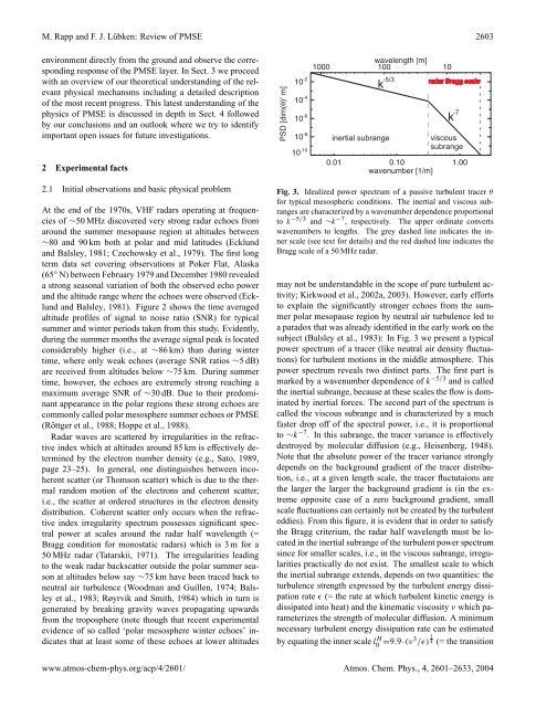Fig. 3. Idealized power spectrum of a passive turbulent tracer θ for typical mesospheric conditions. The inertial and viscous subranges are characterized by a wavenumber dependence proportional to k −5/3 and ∼k −7 , respectively. The upper ordinate converts wavenumbers to lengths. The grey dashed line indicates the inner scale (see text for details) and the red dashed line indicates the Bragg scale of a 50 MHz radar. may not be understandable in the scope of pure turbulent activity; Kirkwood et al., 2002a, 2003). However, early efforts to explain the significantly stronger echoes from the summer polar mesopause region by neutral air turbulence led to a paradox that was already identified in the early work on the subject (Balsley et al., 1983): In Fig. 3 we present a typical power spectrum of a tracer (like neutral air density fluctuations) for turbulent motions in the middle atmosphere. This power spectrum reveals two distinct parts. The first part is marked by a wavenumber dependence of k −5/3 and is called the inertial subrange, because at these scales the flow is dominated by inertial forces. The second part of the spectrum is called the viscous subrange and is characterized by a much faster drop off of the spectral power, i.e., it is proportional to ∼k −7 . In this subrange, the tracer variance is effectively destroyed by molecular diffusion (e.g., Heisenberg, 1948). Note that the absolute power of the tracer variance strongly depends on the background gradient of the tracer distribution, i.e., at a given length scale, the tracer fluctutaions are the larger the larger the background gradient is (in the extreme opposite case of a zero background gradient, small scale fluctuations can certainly not be created by the turbulent eddies). From this figure, it is evident that in order to satisfy the Bragg criterium, the radar half wavelength must be located in the inertial subrange of the turbulent power spectrum since for smaller scales, i.e., in the viscous subrange, irregularities practically do not exist. The smallest scale to which the inertial subrange extends, depends on two quantities: the turbulence strength expressed by the turbulent energy dissipation rate ɛ (= the rate at which turbulent kinetic energy is dissipated into heat) and the kinematic viscosity ν which parameterizes the strength of molecular diffusion. A minimum necessary turbulent energy dissipation rate can be estimated by equating the inner scale l H 0 =9.9·(ν3 /ɛ) 1 4 (= the transition www.atmos-chem-phys.org/acp/4/2601/ Atmos. Chem. Phys., 4, 2601–2633, 2004
Page 1: Atmos. Chem. Phys., 4, 2601-2633, 2
Page 5 and 6: M. Rapp and F. J. Lübken: Review o
Page 33: M. Rapp and F. J. Lübken: Review o

Polar mesosphere summer echoes (PMSE): review of ... - HAL

You also want an ePaper? Increase the reach of your titles

Delete template?

Save as template?