A dynamically-packed planetary system around GJ 667C with ... - ESO

Guillem Anglada-Escudé et al.: Three HZ super-Earths in a seven-planet system
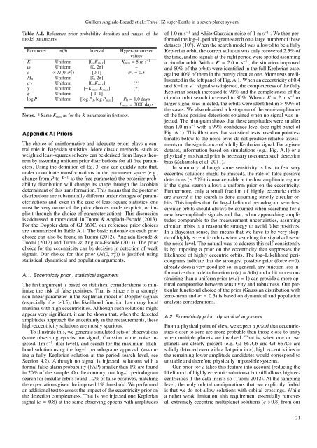
Table A.1. Reference prior probability densities and ranges of the
model parameters
Parameter π(θ) Interval Hyper-parameter
values
K Uniform [0, K max ] K max = 5 m s −1
ω Uniform [0, 2π] –
e ∝ N(0, σ 2 e) [0,1] σ e = 0.3
M 0 Uniform [0, 2π] –
σ J Uniform [0, K max ] (*)
γ Uniform [−K max , K max ] (*)
ϕ Uniform [-1, 1]
log P Uniform [log P 0 , log P max ] P 0 = 1.0 days
P max = 3000 days
Notes. * Same K max as for the K parameter in first row.
Appendix A: Priors
The choice of uninformative and adequate priors plays a central
role in Bayesian statistics. More classic methods -such as
weighted least-squares solvers- can be derived from Bayes theorem
by assuming uniform prior distributions for all free parameters.
Using the definition of Eq. 3, one can quickly note that,
under coordinate transformations in the parameter space (e.g.,
change from P to P −1 as the free parameter) the posterior probability
distribution will change its shape through the Jacobian
determinant of this transformation. This means that the posterior
distributions are substantially different under changes of parameterizations
and, even in the case of least-square statistics, one
must be very aware of the prior choices made (explicit, or implicit
through the choice of parameterization). This discussion
is addressed in more detail in Tuomi & Anglada-Escudé (2013).
For the Doppler data of GJ 667C, our reference prior choices
are summarized in Table A.1. The basic rationale on each prior
choice can also be found in Tuomi (2012), Anglada-Escudé &
Tuomi (2012) and Tuomi & Anglada-Escudé (2013). The prior
choice for the eccentricity can be decisive in detection of weak
signals. Our choice for this prior (N(0, σ 2 e)) is justified using
statistical, dynamical and population arguments.
A.1. Eccentricity prior : statistical argument
The first argument is based on statistical considerations to minimize
the risk of false positives. That is, since e is a strongly
non-linear parameter in the Keplerian model of Doppler signals
(especially if e >0.5), the likelihood function has many local
maxima with high eccentricities. Although such solutions might
appear very significant, it can be shown that, when the detected
amplitudes approach the uncertainty in the measurements, these
high-eccentricity solutions are mostly spurious.
To illustrate this, we generate simulated sets of observations
(same observing epochs, no signal, Gaussian white noise injected,
1m s −1 jitter level), and search for the maximum likelihood
solution using the log–L periodograms approach (assuming
a fully Keplerian solution at the period search level, see
Section 4.2). Although no signal is injected, solutions with a
formal false-alarm probability (FAP) smaller than 1% are found
in 20% of the sample. On the contrary, our log–L periodogram
search for circular orbits found 1.2% of false positives, matching
the expectations given the imposed 1% threshold. We performed
an additional test to assess the impact of the eccentricity prior on
the detection completeness. That is, we injected one Keplerian
signal (e = 0.8) at the same observing epochs with amplitudes
of 1.0 m s −1 and white Gaussian noise of 1 m s −1 . We then performed
the log–L periodogram search on a large number of these
datasets (10 3 ). When the search model was allowed to be a fully
Keplerian orbit, the correct solution was only recovered 2.5% of
the time, and no signals at the right period were spotted assuming
a circular orbit. With a K = 2.0 m s −1 , the situation improved
and 60% of the orbits were identified in the full Keplerian case,
against 40% of them in the purely circular one. More tests are illustrated
in the left panel of Fig. A.1. When an eccentricity of 0.4
and K=1 m s −1 signal was injected, the completeness of the fully
Keplerian search increased to 91% and the completeness of the
circular orbit search increased to 80%. When a K = 2 m s −1 or
larger signal was injected, the orbits were identified in > 99% of
the cases. We also obtained a histogram of the semi-amplitudes
of the false positive detections obtained when no signal was injected.
The histogram shows that these amplitudes were smaller
than 1.0 m s −1 with a 99% confidence level (see right panel of
Fig. A.1). This illustrates that statistical tests based on point estimates
below to the noise level do not produce reliable assessments
on the significance of a fully Keplerian signal. For a given
dataset, information based on simulations (e.g., Fig. A.1) or a
physically motivated prior is necessary to correct such detection
bias (Zakamska et al. 2011).
In summary, although some sensitivity is lost (a few very
eccentric solutions might be missed), the rate of false positive
detections (∼ 20%) is unacceptable at the low amplitude regime
if the signal search allows a uniform prior on the eccentricity.
Furthermore, only a small fraction of highly eccentric orbits
are missed if the search is done assuming strictly circular orbits.
This implies that, for log–likelihood periodogram searches,
circular orbits should always be assumed when searching for a
new low-amplitude signals and that, when approaching amplitudes
comparable to the measurement uncertainties, assuming
circular orbits is a reasonable strategy to avoid false positives.
In a Bayesian sense, this means that we have to be very skeptic
of highly eccentric orbits when searching for signals close to
the noise level. The natural way to address this self-consistently
is by imposing a prior on the eccentricity that suppresses the
likelihood of highly eccentric orbits. The log–Likelihood periodograms
indicate that the strongest possible prior (force e=0),
already does a very good job so, in general, any function less informative
than a delta function (π(e) = δ(0)) and a bit more constraining
than a uniform prior (π(e) = 1) can provide a more optimal
compromise between sensitivity and robustness. Our particular
functional choice of the prior (Gaussian distribution with
zero-mean and σ = 0.3) is based on dynamical and population
analysis considerations.
A.2. Eccentricity prior : dynamical argument
From a physical point of view, we expect a priori that eccentricities
closer to zero are more probable than those close to unity
when multiple planets are involved. That is, when one or two
planets are clearly present (e.g. GJ 667Cb and GJ 667Cc are
solidly detected even with a flat prior in e), high eccentricities in
the remaining lower amplitude candidates would correspond to
unstable and therefore physically impossible systems.
Our prior for e takes this feature into account (reducing the
likelihood of highly eccentric solutions) but still allows high eccentricities
if the data insists so (Tuomi 2012). At the sampling
level, the only orbital configurations that we explicitly forbid
is that we do not allow solutions with orbital crossings. While
a rather weak limitation, this requirement essentially removes
all extremely eccentric multiplanet solutions (e >0.8) from our
21