Benke, A., Huryn, A., Smock, L., Wallace, J. 1999. Length-mass ...

Length-Mass Relationships for Freshwater Macroinvertebrates in North America with
Particular Reference to the Southeastern United States
Author(s): Arthur C. Benke, Alexander D. Huryn, Leonard A. Smock, J. Bruce Wallace
Source: Journal of the North American Benthological Society, Vol. 18, No. 3 (Sep., 1999), pp.
308-343
Published by: The North American Benthological Society
Stable URL: http://www.jstor.org/stable/1468447
Accessed: 11/09/2009 10:49
Your use of the JSTOR archive indicates your acceptance of JSTOR's Terms and Conditions of Use, available at
http://www.jstor.org/page/info/about/policies/terms.jsp. JSTOR's Terms and Conditions of Use provides, in part, that unless
you have obtained prior permission, you may not download an entire issue of a journal or multiple copies of articles, and you
may use content in the JSTOR archive only for your personal, non-commercial use.
Please contact the publisher regarding any further use of this work. Publisher contact information may be obtained at
http://www.jstor.org/action/showPublisher?publisherCode=nabs.
Each copy of any part of a JSTOR transmission must contain the same copyright notice that appears on the screen or printed
page of such transmission.
JSTOR is a not-for-profit organization founded in 1995 to build trusted digital archives for scholarship. We work with the
scholarly community to preserve their work and the materials they rely upon, and to build a common research platform that
promotes the discovery and use of these resources. For more information about JSTOR, please contact support@jstor.org.
The North American Benthological Society is collaborating with JSTOR to digitize, preserve and extend access
to Journal of the North American Benthological Society.
http://www.jstor.org

J. N. Am. Benthol. Soc., 1999, 18(3):308-343
? 1999 by The North American Benthological Society
Length-mass relationships for freshwater macroinvertebrates in North
America with particular reference to the southeastern United States
ARTHUR C. BENKE1'5, ALEXANDER D. HURYN2, LEONARD A. SMOCK3, AND
J. BRUCE WALLACE4
'Aquatic Biology Program, Department of Biological Sciences, Box 870206, University of Alabama,
Tuscaloosa, Alabama 35487-0206 USA
2Department of Biological Sciences, 5722 Deering Hall, University of Maine, Orono,
Maine 04469-5722 USA
3Department of Biology, Virginia Commonwealth University, Richmond, Virginia 23284 USA
4Department of Entomology and Institute of Ecology, University of Georgia, Athens, Georgia 30602 USA
Abstract. Estimation of invertebrate biomass is a critical step in addressing many ecological questions
in aquatic environments. Length-dry mass regressions are the most widely used approach for
estimating benthic invertebrate biomass because they are faster and more precise than other methods.
A compilation and analysis of length-mass regressions using the power model, M (mass) = a L
(length)b, are presented from 30 y of data collected by the authors, primarily from the southeastern
USA, along with published regressions from the rest of North America. A total of 442 new and
published regressions are presented, mostly for genus or species, based on total body length or other
linear measurements. The regressions include 64 families of aquatic insects and 12 families of other
invertebrate groups (mostly molluscs and crustaceans). Regressions were obtained for 134 insect
genera (155 species) and 153 total invertebrate genera (184 species). Regressions are provided for
both body length and head width for some taxa. In some cases, regressions are provided from
multiple localities for single taxa. When using body length in the equations, there were no significant
differences in the mean value of the exponent b among 8 insect orders or Amphipoda. The mean
value of b for insects was 2.79, ranging from only 2.69 to 2.91 among orders. The mean value of b
for Decapoda (3.63), however, was significantly higher than all insects orders and amphipods. Mean
values of a were not significantly different among the 8 insect orders and Amphipoda, reflecting
considerable variability within orders. Reasons for potential differences in b among taxa are explained
with hypothetical examples showing how b responds to changes in linear dimensions and specific
gravity. When using head width as the linear dimension in the power model, the mean value of b
was higher (3.11) than for body length and more variable among orders (2.8-3.3). Values of b for
Ephemeroptera (3.3) were significantly higher than those for Odonata, Megaloptera, and Diptera. For
those equations in which ash-free dry mass was used, % ash varied considerably among functional
feeding groups (3.3-12.4%). Percent ash varied from 4.0% to 8.5% among major insect orders, but
was 18.9% for snails (without shells). Family-level regressions also are presented so that they can be
used when generic equations are unavailable or when organisms are only identified to the family
level. It is our intention that these regressions be used by others in estimating mass from linear
dimensions, but potential errors must be recognized.
Key words: freshwater invertebrates, aquatic insects, length-mass regression, biomass, secondary
production, allometry, dry mass.
Estimation of invertebrate biomass is a critical mass conversion (Burgherr and Meyer 1997).
step in addressing many ecological questions at Length-mass conversions usually are considorganism,
population, community, and ecosys- ered superior to other approaches, primarily betem
levels of organization, regardless of wheth- cause they are faster and more precise (e.g.,
er one is dealing with freshwater, marine, or ter- Burgherr and Meyer 1997). Furthermore, direct
restrial environments. There are 3 basic ap- weighing of preserved organisms is often a
proaches to biomass determination: 1) direct problem because of the loss of dry mass upon
weighing of fresh, frozen, or preserved animals, preservation (e.g., Howmiller 1972, Leuven et al.
2) biovolume determination, and 3) length-dry 1985) Given its many advantages, determination
of biomass from linear dimensions (e.g., total
length or head width) using regression anal-
5 E-mail: abenke@biology.as.ua.edu ysis has been widely used for terrestrial (e.g.,
308

1999] INVERTEBRATE LENGTH-MASS RELATIONSHIPS
309
of length-mass regressions is
Rogers et al. 1976, Schoener 1980, Sample et al. and inventory
1993, H6dar 1996), benthic (e.g., Smock 1980, needed.
North America, a more comprehensive update ship between length and mass (see below).
Meyer 1989, Towers et al. 1994, Burgherr and
Meyer 1997), and planktonic (e.g., McCauley
1984, Kawabata and Urabe 1998) invertebrates.
Thus, the purpose of this paper is to present
a compilation of length-mass relationships for
North American macroinvertebrates, to evaluate
Length-mass regressions can be used for some of these relationships, and to make the
many purposes in ecological studies where equations available to others. Much of this commeasuring
length (or some other linear dimen- pilation is possible because, in the course of consion)
is easier than obtaining mass: 1) they are
useful for estimating biomass in the laboratory
ducting studies on secondary production, we
have accumulated many such equations over the
where growth rates or other bioenergetic vari- past 30 y. We present many unpublished equaables
are measured, 2) they allow estimation of tions that primarily focus on species found in
prey biomass in a the southeastern USA. We also include as
predator gut (particularly
many
equations for head width) even when the prey published length-mass relationships as we
may be torn apart or could find in the literature
partially digested, 3)
to make our
they
presenenable
estimation of population or tation for North America more
community
complete. We
biomass,
have exercised some discretion in our selection
given quantitative length-frequency
data from the field, 4) they are useful in estab- of regressions from the literature.
lishing size-specific mass for most secondary
production methods, 5) they allow for more
Basic length-mass model
comprehensive comparisons of invertebrate
populations within and between habitats and Length-mass equations in the context of this
ecosystems, and 6) they provide more paper will refer energet-
only to those that predict mass
ically based response variables for as a power function of a linear dimension
asking ques-
(partions
about interspecific relationships (Benke
ticularly body length and head width):
1993).
M = aLl' [1]
The most common approach in developing where M is
length-mass equations for freshwater macroin-
organism mass (mg), L is any linear
dimension
vertebrates is to describe mass as a power func-
(mm), and a and b are constants.
tion of a linear dimension. The power function Equation 1 often is converted to a linear form
usually provides a better fit to the data than
by using a logarithmic transformation:
most other mathematical formulations (e.g.,
loglo M = log a + b log L [2]
Wenzel et al. 1990). Unfortunately, equations
predicting mass from linear dimensions are
or
widely scattered in the literature. Many inves-
log, M = lnM = lna + b lnL [3]
tigators report the development of such relationships,
particularly in studies of For equations 2 and 3, the exponent b of the
secondary propower
model becomes the slope of a linear reduction,
but often the equations are not actually
gression,
presented in the publications. It is log,, a and In a are Y intercepts
becoming (i.e., the value of log,, M or In M when log,, L
widely recognized that there is a need to make or In L = 0, which occurs when L = 1). In this
such regressions available for others to use. For
example, recent paper,
compilations of such informa-
logarithmically trans-
formed.
tion have been presented for Europe (Meyer Both the power curve and the log,,-trans-
1989, Wenzel et al. 1990, Burgherr and Meyer formed linear regression are illustrated for the
1997) and New Zealand (Towers et al. 1994). The
aquatic megalopteran Corydalus cornutus (Fig. 1).
only compilation of such regressions for North The statistics for this large predaceous insect are
American macroinvertebrates was completed by interesting for 2 reasons. First, the range in mass
Smock (1980), which contained specific equa- from 1st to final instar may be the highest of
tions for 43 species/genera from 31 insect fam- any aquatic insect (ca x10,000). Second, the exilies,
and 8 order-level equations for insects. ponent b (or slope of the linear regression) =
Given the paucity of specific regressions for 3.0, which represents a perfect cubic relation-

310 A. C. BENKE ET AL.
Total length (mm)
[Volume 18
0 10 20 30 40 50 60
400
300
c0
E
U)
-a (3
{3
0
OI o1
100
E
200 vc
E
"lf
0.5 1 1.5 2 2.5 3
Log total length (mm)
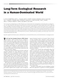
FIG. 1. Length-mass curves for the aquatic megalopteran Corydalus cornutus from Coastal Plain rivers in
Georgia, using both linear (filled squares) and logarithmic (logio, open circles) scales. The power equation is
DM = 0.0018 L 2.997, where DM = dry mass and L = body length (r2 = 0.95, n = 82, and lengths ranged from
2.4 to 62.0 mm).
0
For any length-mass equation, mass is predicted
by taking a known length (L) to the power
b and multiplying by a. For example, the dry
mass (DM) of C. cornutus having a length of 30
mm would be estimated as DM = 0.0018 x
302997 = 48.1 mg.
Methods
New equations from the eastern USA
Invertebrates for regression analysis were collected
from 1968 through 1998 from ponds,
streams, rivers, and wetlands in Alabama, Georgia,
Maine, North Carolina, South Carolina, and
Virginia. For each population, -1 linear measurements
were made of total length, head
width, or some other taxon-specific dimension
such as carapace length of crayfish. Most invertebrates
(i.e., those

1999] INVERTEBRATE LENGTH-MASS RELATIONSHIPS
311
Ash-free dry mass (AFDM) was used in regressions
estimated by A. D. Huryn and J. B. Wallace.
After DM was measured, invertebrates
were ashed in a muffle furnace at 500?C. Ash
mass was then subtracted from DM to obtain
AFDM.
We provide the following statistics for most of
the regressions presented from our original
data: a ? 1 SE, b ? 1 SE, coefficient of determination
(r2), range of the linear measurement,
number of data points in the regression (n), and
collection location (i.e., state). For most of the
equations estimated by A. D. Huryn and J. B.
Wallace, the % ash also is provided so that one
can estimate DM as well as AFDM (see Huryn
et al. 1994 for details) as follows:
100
DM = AFDM 100 [4]
100 - % ash'
A. D. Huryn's regressions for snails (Elimia spp.)
are revisions of those found in Huryn et al.
(1994). Percent ash for snails is presented both
with and without shells.
The ability to convert DM to AFDM and vice
versa would be very useful to investigators who
may wish to use any of these equations. Furthermore,
it is of biological interest to determine
whether there are differences in ash content
among invertebrates with different feeding
modes and among major taxonomic groups. We
therefore separated those organisms with
AFDM equations into functional groups (filtering
collectors, scrapers, shredders, gathering
collectors, and predators; Merritt and Cummins
1996), and calculated mean values of % ash. We
also calculated mean % ash for major taxonomic
groups.
Published equations and selection criteria
We established several restrictive criteria in
the selection of published regressions: 1) Equations
must have been based on the power model
described above. 2) Mass must have been ex-
pressed as either DM or AFDM. Regressions
based on live (= wet) mass were not included.
3) Dry mass must have been determined from
either fresh animals or animals preserved in formalin.
4) There was sufficient information about
the units of the linear dimension and mass, and
whether standard procedures were followed
(e.g., type of preservative used). 5) Equations
obtained from the literature made biological
sense. Published equations that generated unrealistic
numbers and that could not be corrected
were excluded.
We attempted to present the same statistics
for the literature values as for our original equations.
However, although many published re-
gressions included n and r2, most did not include
standard errors of a and b. All equations
are presented using mg for DM and mm for
length; other units (e.g., g, cm, jm) were converted
to these standard units to obtain the final
form of the equation. We used a one-way analysis
of variance (ANOVA) and, if significant, a
Tukey-Kramer test to compare the mean values
of b among major insect and crustacean orders.
Homogeneity of variances was tested with Bartlett's
test. For those orders in which b was not
significantly different, the same statistical test
was followed for the a value (prior to analysis,
all a values in AFDM regressions 1st were converted
to DM). Tests of the a value were restricted
to orders with no differences in b values because
of the likelihood that a is not independent
of b. ANOVA and Tukey-Kramer tests also were
used to compare mean values of b for head
width among insect orders, and to compare differences
in % ash content among different functional
feeding groups and among major taxonomic
groups.
Although we focus on the need for genusand
species-level regressions, some investigators
may require the use of family-level regressions.
Such regressions might be useful when genuslevel
regressions are unavailable, or when individuals
are identified only to the family level.
To provide such equations, we estimated mean
values of a and b for equations based on total
body length for each insect family, and other
major groups. All a values based on AFDM first
were converted to DM.
Regression equations
Results
We present a total of 442 new and published
regressions based on either total body length or
a shorter dimension (e.g., head width) in Appendices
1, 2, and 3. Sixty-four families of aquatic
insects and 12 families of other invertebrates
are represented by at least 1 regression, with all
but Empididae and Sciaridae (Diptera) having
at least 1 genus-level equation per family (Table

312 A. C. BENKE ET AL.
[Volume 18
TABLE 1. Numbers of families, genera, and species
of invertebrates for which length-mass regressions are
presented in Appendices 1, 2, and 3. For the insect
taxa, the total number of families from North America
within each order is also presented in parentheses
(based on Merritt and Cummins 1996).
No. of No. of No. of
Taxonomic group families genera species
Insecta
Ephemeroptera 12 (21) 29 34
Odonata 7 (9) 17 18
Plecoptera 9 (9) 24 29
Hemiptera 3 (18) 4 4
Megaloptera 2 (2) 3 3
Trichoptera 14 (22) 24 29
Lepidoptera 1 (5) 1 1
Coleoptera 7 (25) 12 12
Diptera 9 (27) 23 25
Total Insecta 64 (139) 134 155
Mollusca 4 7 12
Crustacea 7 9 15
Turbellaria 1 2 2
Total Invertebrates 76 153 184
1). Most of the families of Ephemeroptera,
Odonata, Plecoptera, Megaloptera, and Trichoptera
found in North America (Merritt and Cummins
1996) are represented, even though our
own analyses focused only on 6 eastern states.
Thus, orders found primarily in lake, stream,
and river benthos are well represented. However,
the Hemiptera, Lepidoptera, Coleoptera,
and Diptera, containing several families with
semi-aquatic taxa, had a poor family-level representation.
Regressions were found for 134 insect
genera and 155 species. Considering total
invertebrates, 76 families, 153 genera and 184
species are represented.
The number of equations reported in the Appendices
exceeded the total number of represented
taxa because there were often several
equations per taxon for a given genus (e.g., Bae-
tis spp.) or species (e.g., Corydalus cornutus). In
some cases, taxa had regressions for both length
and head width; in others taxa had regressions
from >1 state and >1 stream, river, or lake
within a state (e.g., Appendix 2, several Elimia
spp.); and in still others there were regressions
from >1 site within the same stream, river, or
lake (e.g., Appendix 2, Hornbach et al. 1996).
Variability in length-mass constants among
macroinvertebrates
There were no significant differences in mean
b values for body length among all insect orders
and the Amphipoda (Table 2, Fig. 2; ANOVA
and Tukey-Kramer test; variances homogeneous).
However, the mean b for Decapoda
(3.626 ? 0.084) using carapace length was significantly
higher than mean b values for all other
TABLE 2. Mean values of b and a from length-mass regressions for the major insect and crustacean orders
using total length (Appendix 1). Equations using a dimension other than total length (e.g., thorax length) were
not used in calculating means, except for Decapoda (carapace length; included only in ANOVA for b). If letters
under signif. (c and d) are the same for any 2 taxa, then means were not significantly different between taxa
(ANOVA and Tukey-Kramer test, p > 0.05). Min. and max. indicate the minimum and maximum values of b
and a from all regressions for that order. n = number of equations used for each order. Galerucella nymphaeae
was excluded from the Coleoptera estimates because it is primarily terrestrial and has a and b values that
deviate substantially from most other taxa.
Order n b + 1 SE Signif. Min. Max. a + 1 SE Signif. Min. Max.
Decapoda 9 3.626 + 0.084 c 3.357 4.066 0.0147 + 0.0030 0.0041 0.0307
Amphipoda 7 3.015 + 0.087 d 2.740 3.404 0.0058 + 0.0014 c 0.0010 0.0120
Coleoptera 9 2.910 + 0.117 d 2.311 3.521 0.0077 ? 0.0021 c 0.0011 0.0181
Trichoptera 34 2.839 + 0.060 d 2.389 4.179 0.0056 + 0.0006 c 0.0005 0.0180
Megaloptera 7 2.838 + 0.053 d 2.691 3.001 0.0037 + 0.0006 c 0.0018 0.0062
Ephemeroptera 54 2.832 + 0.046 d 2.252 4.140 0.0071 + 0.0007 c 0.0001 0.0257
Odonata 18 2.792 + 0.052 d 2.239 3.124 0.0078 + 0.0009 c 0.0015 0.0180
Plecoptera 36 2.754 + 0.041 d 1.950 3.232 0.0094 + 0.0017 c 0.0019 0.0538
Hemiptera 4 2.734 ? 0.068 d 2.596 2.904 0.0108 + 0.0032 c 0.0031 0.0169
Diptera 43 2.692 + 0.052 d 2.091 3.830 0.0025 + 0.0003 c 0.0002 0.0066
All Insects 205 2.788 + 0.022 1.95 4.179 0.0064 + 0.0004 0.0001 0.0538

1999] INVERTEBRATE LENGTH-MASS RELATIONSHIPS
313
0)
E Ov
U,
CO
0
E
>.
Hemiptera
Plecoptera
Odonata
Coleoptera
Ephemeroptera
Amphipoda
Trichoptera
Megaloptera
Diptera
1 10 100
Length (mm)
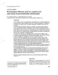
FIG. 2. Comparison of composite length-mass relationships for the major orders of aquatic insects and
crustaceans. All equations are of the form DM = a Lb, where DM = dry mass and L = body length. Neither
of the fitted coefficients (a and b) were significantly different among the 8 insect orders and the Amphipoda.
The slope (b) for the Decapoda was significantly different from all other orders. Because the decapod equation
was based on carapace length, not total body length, comparison of the a value for decapods with other a
values was irrelevant. Length of each line indicates the maximum value for each order.
orders. Mean b for all insect orders was 2.788 ?
0.022 (n = 205), with a range in means of b from
only 2.69 to 2.91 among orders.
Because there were no differences in mean b
among insect orders and amphipods, we conducted
the same multiple-comparison test to determine
whether there were differences in a. All
a values based on AFDM 1st were converted to
DM. Although the highest mean values of a (Hemiptera
and Plecoptera) were several times
higher than the lowest value (Diptera), the variability
within orders was too large to detect
any significant differences among orders (Table
2, Fig. 2). Variances were heterogeneous for this
ANOVA, even after data transformation. Therefore,
data were reanalyzed using the Games-
Howell method designed for cases when variances
are heterogeneous (Sokal and Rohlf 1995).
The results were the same as the original AN-
OVA, with no differences among the mean a values.
The variability of a within orders can be
seen from examination of their coefficients of
variation (CV), which ranged from 43 to 108%.
In contrast, CV for b values ranged from only 5
to 13%.
The mean b for head-width equations using
all insect orders was 3.111 ? 0.037 (n = 147,
Table 3). However, b for head width differed
more among orders than b for body length.
Mean values of b for head width ranged from
2.8 (Diptera) to 3.3 (Ephemeroptera), and differences
were highly significant (ANOVA, variances
homogeneous, p < 0.001). Ephemeroptera b
was significantly higher than values for Odonata,
Megaloptera, and Diptera (Tukey-Kramer
test). Trichoptera b was significantly higher than
the value for Diptera.
No attempt was made to conduct statistical
analyses on the equations for molluscs (Appendix
2) because the total number of species listed
was relatively low, and the length dimension
represented 3 different and therefore incomparable
measures: maximum shell length, maximum
shell width (gastropod only), or maximum
shell width at aperture (gastropods only).
Sixty-one family-level regressions for insect
larvae were estimated (Table 4) using mean a
and b values based on total body length (Appendix
1). Regressions included 12 families of
Ephemeroptera, 7 Odonata, 9 Plecoptera, 2 Megaloptera,
14 Trichoptera, 1 Lepidoptera, 4 Co-
leoptera, and 9 Diptera. Only 9 of these families
had mean b values >3. Regressions were also
estimated for 3 major crustacean orders and

314 A. C. BENKE ET AL.
[Volume 18
TABLE 3. Mean values of b for length-mass regressions for the major insect orders using head width (Appendix
3). If letters under signif. (c, d, e) are the same for any 2 taxa, then means are not significantly different
between taxa (ANOVA and Tukey-Kramer text, p > 0.05). Min. and max. indicate the minimum and maximum
values of b from all regressions. Galerucella nymphaeae was excluded from the Coleoptera estimates because it is
primarily terrestrial and has a and b values that deviate substantially from most other taxa.
n b + 1 SE Signif. Min. Max.
Ephemeroptera 32 3.319 + 0.053 c 2.764 4.111
Trichoptera 30 3.252 ? 0.088 cd 2.284 4.580
Coleoptera 8 3.140 ? 0.154 cde 2.645 3.794
Plecoptera 39 3.094 ? 0.073 cde 2.000 4.000
Odonata 17 2.871 + 0.092 de 2.401 3.592
Megaloptera 9 2.838 + 0.089 de 2.474 3.256
Diptera 12 2.791 + 0.160 e 2.311 4.347
Turbellaria. Two of 3 b values were >3 for crustaceans.
Variability of mass for a given linear dimension
To illustrate the variability associated with individual
length-mass regressions, we have chosen
a holometabolous insect, the caddisfly Hydropsyche
elissoma (Fig. 3). It is apparent that the
last 4 instars fall within a narrow range of headwidth
values when plotting head width vs mass
(Fig. 3A). With each molt, dimensions of sclerotized
body parts (e.g., head width) rapidly in-
creased by -50%. The average caddisfly volume
would therefore be expected to triple at molting
(i.e., 1.53 - 3), even though dry mass will decline
slightly (from loss of exuviae). This prediction
is consistent with the observation that
variation of DM within an instar is -3-fold (Fig.
3A). In spite of this clumping of head-width values
and relatively large differences in mass
within an instar, there was still a highly significant
regression with narrow 95% confidence
limits (CL) and a high r2. In contrast, the body
length plot for the same species showed no
clumping of instars (Fig. 3B), probably because
growth of the unsclerotized abdomen was more
continuous than growth of the head. Nonetheless,
r2 and 95% CL were similar for both regressions.
Percent ash
Percent ash was estimated for 80 of the regressions
in Appendices 1, 2, and 3, and mean
% ash was calculated for functional feeding
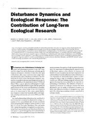
groups and taxonomic groups. Mean values of
% ash varied considerably among functional
feeding groups (Fig. 4A). Filtering collectors
and scrapers had mean values ca 11-12%,
shredders and gathering collectors ca 5-6%, and
predators ca 3%, possibly indicating differences
in the material ingested by species of different
functional feeding groups. Although mean values
of % ash were significantly different among
functional groups (ANOVA, p < 0.05), the Tukey-Kramer
test only found that the predator
value was significantly lower than either scrapers
or filtering collectors, and the other functional
groups were not significantly different
from one another (square root arcsin transformation
of percentages, variances homogeneous).
Mean values of % ash varied from only 4.0%
to 8.5% among major insect orders (Fig. 4B).
Gastropoda, Decapoda, and Lepidoptera were
noticeably higher (>17%), but the latter 2 only
had a single measurement and could not be
used in statistical analyses. Mean values of %
ash were significantly different among those
groups represented by >1 equation (ANOVA, p
< 0.05, square root arcsin transformation of percentages,
variances homogeneous). The mean %
ash content for Plecoptera and Diptera was significantly
lower than ash content for Trichoptera
and Gastropoda (Tukey-Kramer test). The mean
ash contents for Ephemeroptera, Coleoptera,
and Trichoptera were not significantly different
from one another, but all were significantly lower
(4.0-8.5%) than the ash content for Gastropoda
(18.9%, without shell).
Discussion
Our compilation and analysis of invertebrate
length-mass regressions for North America en-

1999] INVERTEBRATE LENGTH-MASS RELATIONSHIPS
315
abled us to describe the variability in such relationships
within and among taxonomic
groups, and to provide other investigators with
equations that may prove useful in their own
studies. Therefore, we will attempt to explain
some of the observed variability and offer some
guidance in the use of these equations.
Variability in length-mass constants among
macroinvertebrates
Inspection of the equations for all invertebrate
groups reveals that the exponent b is often close
to a value of 3 (Appendices 1, 2, and 3). The
shape of the animals and their specific gravity
must remain exactly the same throughout larval
development for the expected value of b to be
exactly 3. However, the shape of virtually all
aquatic invertebrates changes somewhat as they
grow, and specific gravity does not remain constant.
For insects, the mean value of b for body
length is actually somewhat

316
A. C. BENKE ET AL. [Volume 18
TABLE 4. Higher-level length-mass equations (DM = a Lb, where DM is dry mass [mg], L is total body
length [mm], and a and b are constants) for Turbellaria (class), crustaceans (order), and insect larvae (family).
For Decapoda, L = carapace length. All a and b values are means calculated from individual taxa within a
group (Appendix 1). n = the number of equations used in calculating the mean. Note that several equations
are based on only a single equation from Appendix 1 (i.e., n = 1). See Appendix 1 for details.
Taxon b ? 1 SE a + 1 SE n
Turbellaria 2.168 ? 0.016 0.0082 ? 0.0013 3
Crustacea
3.015 + 0.087
0.0058 + 0.0014
7
3.626 ? 0.084
0.0147 + 0.0030
9
2.948 ? 0.163
0.0054 ? 0.0018
2
Amphipoda
Decapoda
Isopoda
Ephemeroptera
Ameletidae
Baetidae
Baetiscidae
Caenidae
Ephemerellidae
Ephemeridae
Heptageniidae
Isonychiidae
Leptophlebiidae
Polymitarcyidae
Siphlonuridae
Tricorythidae
Odonata
Aeshnidae
Calopterygidae
Coenagrionidae
Cordulegastridae
Corduliidae
Gomphidae
Libellulidae
Plecoptera
Capniidae
Chloroperlidae
Leuctridae
Nemouridae
Peltoperlidae
Perlidae
Perlodidae
Pteronarcyidae
Taeniopterygidae
Hemiptera
Corixidae
Gerridae
Veliidae
Megaloptera
Corydalidae
Sialidae
Trichoptera
Brachycentridae
Glossosomatidae
Helicopsychidae (case width)
Hydropsychidae
Lepidostomatidae
Leptoceridae
2.588
2.875 + 0.131
2.905
2.772 + 0.069
2.676 + 0.131
2.764 + 0.043
2.754 + 0.039
3.043 + 0.124
2.686 + 0.082
3.050
3.446 + 0.455
3.194 + 0.028
2.813
2.742
2.785 + 0.119
2.782
2.787 + 0.050
2.787 - 0.147
2.809 + 0.134
2.562 + 0.100
2.724
2.719 + 0.025
2.762 ? 0.107
2.737 ? 0.116
2.879 + 0.092
2.742 + 0.043
2.573 + 0.273
2.655 + 0.058
2.904
2.596
2.719 ? 0.058
2.873 + 0.069
2.753 ? 0.048
2.818 + 0.317
2.958 + 0.070
3.096
2.926 ? 0.151
2.649
3.212
0.0077
0.0053 + 0.0010
0.0116
0.0054 ? 0.0008
0.0103 + 0.0025
0.0034 ? 0.0009
0.0108 + 0.0014
0.0031 + 0.0000
0.0047 + 0.0006
0.0020
0.0027 ? 0.0025
0.0061 ? 0.0032
0.0082
0.0050
0.0051 ? 0.0036
0.0067
0.0096 ? 0.0015
0.0088 ? 0.0025
0.0076 ? 0.0019
0.0049 ? 0.0004
0.0065
0.0028 ? 0.0003
0.0056 ? 0.0010
0.0170 + 0.0029
0.0099 ? 0.0030
0.0196 ? 0.0118
0.0324 ? 0.0260
0.0072 ? 0.0012
0.0031
0.0150
0.0126 ? 0.0043
0.0037 + 0.0009
0.0037 - 0.0006
0.0083 + 0.0056
0.0082 ? 0.0017
0.0125
0.0046 ? 0.0007
0.0079
0.0034
1
9
1
4
8
4
15
2
5
1
3
2
1
1
2
1
3
5
5
3
1
2
3
2
13
7
2
4
1
1
2
5
2
3
2
1
10
1
1

1999] INVERTEBRATE LENGTH-MASS RELATIONSHIPS
317
TABLE 4.
Continued.
Taxon b + 1SE a 1 SE n
Limnephilidae 2.933 + 0.065 0.0040 + 0.0008 4
Odontoceridae 2.988 + 0.253 0.0077 + 0.0005 2
Philopotamidae 2.511 + 0.074 0.0050 + 0.0000 3
Phryganeidae 2.811 0.0054 1
Polycentropodidae 2.705 + 0.174 0.0047 + 0.0024 2
Psychomyiidae 2.873 0.0039 1
Rhyacophilidae 2.480 0.0099 1
Sericostomatidae 2.741 0.0074 1
Lepidoptera
Pyralidae 2.918 0.0033 1
Coleoptera
Chrysomelidae 3.111 0.039 1
Elmidae 2.879 + 0.177 0.0074 + 0.0025 6
Psephenidae 2.906 + 0.023 0.0123 + 0.0041 2
Ptilodactylidae 3.100 0.0012 1
Diptera
Athericidae 2.586 0.0040 1
Blephariceridae 3.292 0.0067 1
Ceratopogonidae 2.469 + 0.213 0.0025 + 0.0011 3
Chironomidae 2.617 + 0.067 0.0018 + 0.0004 17
Empididae 2.546 + 0.110 0.0054 + 0.0012 2
Sciaridae 2.091 0.0042 1
Simuliidae 3.011 + 0.153 0.0020 + 0.0006 8
Tabanidae 2.591 0.0050 1
Tipulidae 2.681 + 0.055 0.0029 + 0.0007 9
relatively high b values for decapod equations
in Appendix 1 suggest that both male and female
chelipeds may have accelerated growth, although
rates would be greater in males than females.
Finally, most b values for molluscs were
close to 3, with several slightly above or slightly
below 3, suggesting little change in shape or
specific gravity relationships described above.
It is difficult to compare our a values with
those from the literature because a probably is
not independent of b. However, comparisons of
the plotted lines themselves provide some interpretive
value. Our mean values of a (0.0064) and
b (2.788) for all insects (Table 2) produced a line
that was reasonably similar to the line for all
aquatic insects (a = 0.019, b = 2.46) generated
by Smock (1980) from North Carolina (Fig. 5).
Predicted values tend to converge toward the
larger length categories (i.e., 10-50 mm). The
line for all aquatic insects (a = 0.0027, b = 2.79)
generated by Burgherr and Meyer (1997) for
Central Europe has a slope that is identical to
our own (Fig. 5). However, their lower a value
results in a line that falls below our line and the
one produced by Smock (1980), and would estimate
a lower mass for a given length. This discrepancy
may be a result of differences in the
individual taxa that were used to generate the
regressions, and should serve as a warning that
generalized equations may be inaccurate if applied
to individual taxa.
Our all-insects regression line and those of
Smock (1980) and Burgherr and Meyer (1997)
each fell below the regression line for terrestrial
(presumably adult) insects (a = 0.0305, b = 2.62)
produced by Rogers et al. (1976). Other general
length-mass regressions for adult terrestrial insects
by Schoener (1980), Sample et al. (1993),
and Hodar (1996) also were above our regression
for aquatic insects. The higher mass predicted
by regressions for terrestrial insects suggests
either a higher specific gravity or a broader
body than is found in aquatic insects. A higher
specific gravity for terrestrial adults could be
a result of heavier sclerotization. Alternatively,
morphological differences between adults and
larvae, such as the presence of wings and genitalia,
could partially account for heavier adults.

318 A. C. BENKE ET AL.
[Volume 18
0,
E
05 Hydropsyche elissoma
.5
A
0-
-0.5-
-1.0 -
Un -1.5
E
>1 O3
o 0.5
-J
0
-0.5
-1.0
-' ?-
I I I .
B
/
.I . . . I
I
,-
'
lg DM
'
2 .5 o
.2log DM = 2.580 log HW + 0.083
.r2 n an n - 9Fi rannn - n A
\r = u.vu, I = ;- , lrang = U.4 -1
I.")
I I I .
I . . .
-0.4 -0.3 -0.2 -0.1
Log head width (mm)
I
(sr
. . . . I . .
log DM = 2.491 log BL - 2.236
,
.I
0
.
* , I
(r2 = 0.93, n = 26, range = 2.4 -10.0)
-1.5 I I I I I
0.4 0.5 0.6 0.7 0.8 0.9 1
Log body length (mm)
FIG. 3. Length-mass regressions for head width
(A) and body length (B) for Hydropsyche elissoma from
the Satilla River, Georgia. n = number of data points,
range = range of values for length or width, DM =
dry mass, HW = head width, and BL = body length.
Dashed lines represent 95% confidence limits.
Variability of mass for a given linear dimension
It is important to recognize that when freshwater
arthropods molt, they suddenly increase
their body volume without increasing their DM
(the cast exuviae actually represents a loss of
mass). This phenomenon introduces variability
into length-mass regressions, because animals
collected for weighing may have just molted or
be close to molting. Thus, animals of the same
body dimensions may vary considerably in their
DM. In spite of this natural variability, the value
of b will not necessarily deviate from 3 unless
there is a progressive change in average specific
gravity with size.
Insect larvae belonging to the holometabolous
orders (= Endopterygota) generally have greater
within-instar variability in DM than those in
the hemimetabolous orders (= Exopterygota),
because most Holometabola tend to have fewer
instars and thus increase more in linear dimensions
(and mass) from 1 instar to the next than
the Hemimetabola (Cole 1980, Butler 1984,
Filtering collectors
Scrapers
Shredders
Gathering collectors
Predators
Decapoda
Gastropoda
Lepidoptera
Trichoptera
Coleoptera
Ephemeroptera
Diptera
A
3.3(10)
4.7 (5)
) 2 4 6 8 10 12 14 16
B * 30.6(1)
-*- 8.5(9)
-- 8.0(3)
-- 7.2(14)
* 4.2(12)
5.8 (9)
-0
--- 18.9(8)
* 17.7(1)
12.4(4)
11.0 (25)
--t
Plecoptera * 4.0 (9)
.......
0 5 10 15 20 25 30 35
% dry mass composed of ash
FIG. 4. Percentage of dry mass composed of ash
for aquatic invertebrates in different functional feeding
groups (A), and in different taxonomic groups (B).
Data are from Appendices 1, 2, and 3. Error bars are
+ 1 SE. Value associated with each data point is mean
% ash and n is in parentheses.
Hutchinson et al. 1997). To accomplish the large
increase in mass after molting, much of the cuticle
of holometabolous insects remains unsclerotized
and undifferentiated. For example, when
larval caddisflies molt, the initially soft cuticle
of their heads rapidly reaches its instar-specific
width and quickly hardens (Fig. 3A), but the
undifferentiated cuticle of their abdomen is
somewhat extensible and facilitates more continuous
growth and as much as a tripling of
mass (Fig. 3B). Sclerotized cuticle such as the
head capsule is lost at molting, but the unsclerotized
cuticle (i.e., endocuticle) is largely reabsorbed,
which is energetically economical for
larval development (Chapman 1982). In contrast
to the Holometabola, most growth of the more
completely sclerotized Hemimetabola occurs at
molting when new soft cuticle is produced. For
example, dragonflies usually have -10-12 in-
stars, increase their linear dimensions by -28%
at each molt, and approximately double their
volume (A. C. Benke, unpublished data). Mayflies
usually have 15-25 instars (Butler 1984). If
they increase their linear dimensions by -10%
at each molt, volume only increases by -33%.

1999] INVERTEBRATE LENGTH-MASS RELATIONSHIPS 319
TABLE 5. Hypothetical examples of the effect of changes in body shape and specific gravity (mass/volume)
on the exponent (slope) of length-mass equations, M = a Lb, where M = body mass, L = body length (or head
width in example 4), a = constant coefficient, and b = exponent. Mass is calculated from linear dimensions as
width x height x length, assuming a cuboid shape, and assuming specific gravity = 1 unless otherwise
specified. Examples are: 1) constant body shape in which all dimensions increase by a factor of 1.2 from one
size class (1, 2, 3, 4) to the next, 2) changing body shape in which width and height increase by a factor smaller
than length, 3) constant body shape in which specific gravity declines with body size, 4) an equation based on
head width, with a constant body shape, except that head width increases by a factor smaller than body length,
5) constant, but flattened, body shape in which all dimensions increase by a factor of 1.2, and 6) flattened body
in which height is constant, but length and width increase by a factor of 1.2.
Size class
1 2 3 4
1) Constant body shape
Length (x 1.2) 5.00 6.00 7.20 8.64
Width (x 1.2) 1.00 1.20 1.44 1.73
Height (x 1.2) 1.00 1.20 1.44 1.73
Mass 5.00 8.64 14.93 25.80
a = 0.040 b = 3.000
2) Declining body width and height
Length (x 1.2) 5.00 6.00 7.20 8.64
Width (x 1.1) 1.00 1.10 1.21 1.33
Height (x 1.1) 1.00 1.10 1.21 1.33
Mass 5.00 7.26 10.54 15.28
a = 0.187 b = 2.040
3) Constant shape, declining specific gravity
Length (x 1.2) 5.00 6.00 7.20 8.64
Width (x 1.2) 1.00 1.20 1.44 1.73
Height (x 1.2) 1.00 1.20 1.44 1.73
Volume 5.00 8.64 14.93 25.80
Mass/volume (x 0.98) 1.100 1.078 1.056 1.035
Mass 5.500 9.31 15.77 26.70
a = 0.053 b = 2.889
4) Constant shape, declining head width
Head width (X 1.15) 1.2 1.38 1.59 1.83
Length (x 1.2) 5.00 6.00 7.20 8.64
Width (x 1.2) 1.00 1.20 1.44 1.73
Height (x 1.2) 1.00 1.20 1.44 1.73
Mass 5.00 8.64 14.93 25.80
a = 2.465 b = 3.886
5) Constant (flat) body shape
Length (x 1.2) 5.00 6.00 7.20 8.64
Width (x 1.2) 2.00 2.40 2.88 3.46
Height (x 1.2) 0.40 0.48 0.58 0.69
Mass 4.00 6.92 11.94 20.64
a = 0.032 b = 3.000
6) Flattened body, constant height
Length (x 1.2) 5.00 6.00 7.20 8.64
Width (x 1.2) 2.00 2.40 2.88 3.46
Height (x 1.0) 0.40 0.40 0.40 0.40
Mass 4.00 5.76 8.29 11.94
a = 0.160 b = 2.000

320 A. C. BENKE ET AL.
[Volume 18
c3
E
15)
(/
E
-
0
-j
3-
This paper Terrestrial
2- Smock (1980)
Burgherr and Meyer (1997) .. .
1- .................. .' ,,
Rogers et al. (1976) . ./.
.- /J'-
~''
* /
0-
.'/ /
... /
/
-1
,.///
-2 -
j./'
-3 . E . I
. . . ? I ? I !
0 0.5 1
Log body length (mm)
FIG. 5. Comparison of general length-mass equations
of insects, including aquatic insects from North
Carolina (Smock 1980), Central Europe (Burgherr and
Meyer 1997), and North America (this paper), and terrestrial
insects from a North American grassland in
Washington state (Rogers et al. 1976). All equations
are of the form log1, DM = b logo1 BL + log10 a, where
DM = dry mass, BL = body length, and a and b are
fitted constants. Values of a and b for each equation
are presented in the text.
Thus, it is important to recognize that the deviation
of individual data points from the
length-mass regression line (as indicated by r2)
is partly the result of inherent variability within
an instar rather than measurement error. Furthermore,
using a length-mass regression to estimate
mass for a single individual of a holometabolous
taxon may result in a 50-100% error.
For example, the highest value (2.65 mg) of the
5th instar used in the head-width regression for
Hydropsyche elissoma is 71% higher than the value
(1.55 mg) predicted by the regression (Fig.
3A). Variation of mass within a hemimetabolous
instar also can be substantive, but is likely to be
smaller than for holometabolous orders. For example,
Wenzel et al. (1990) warned that a 20%
error from a length-mass regression can be expected
because of within-instar variation in
mass for Ephemeroptera. Considering such potential
errors, caution should be exercised if such
regressions are used for estimating mass of an
individual animal. In contrast, their utility is
greater for studies in which one is seeking a
mean value for large numbers of animals found
in a single length class.
Dry mass vs AFDM
We believe that equations based on AFDM are
more accurate than those using DM (which includes
ash content). The use of AFDM eliminates
the possibility that some gut contents may
contain inorganic materials or that inorganic silt
may adhere to exoskeletons, biasing mass determinations
with material that is not tissue.
However, estimating AFDM is more time consuming
than estimating DM, and most investi-
gators do not go to the extra trouble. Whether
the extra work involved is worth the effort is
certainly debatable. Our % ash estimates (Fig. 4)
should enable anyone to convert values estimated
from a DM equation to AFDM values and
vice versa. There appeared to be better discrimination
of % ash among taxonomic groups than
among functional groups. However, the func-
tional group conversions may prove useful as
well, particularly for species where taxonomic
conversions are missing. Most of our % ash estimates
were somewhat lower than the 10% approximated
by Waters (1977) for zoobenthos
and zooplankton.
Although most investigators use units of DM
or AFDM, approximate conversions to energy,
wet mass, and C are available (e.g., Waters 1977).
More recently, Wenzel et al. (1990) estimated
that % C ranged from 45.1 to 48.2% of DM for
mayflies in Germany. If AFDM is -93% of DM
for mayflies (Fig. 4), then the Wenzel et al.
(1990) estimate of % C would range from 48.5
to 51.8% of AFDM. In addition, A. D. Huryn
(unpublished data) estimated that the mean C
content of AFDM was 47.8% for various freshwater
invertebrates (molluscs, oligochaetes, am-
phipods, and insects) in New Zealand. Thus,
mean C content of AFDM appears to be consis-
tently close to 50% for freshwater invertebrates.
A. D. Huryn (unpublished data) also estimated
that AFDM consisted of 10.4% N.
Usefulness of published length-mass regressions
We hope that our compilations of equations
are helpful to other investigators in their own
research, but we urge caution in their application.
How does one select the most appropriate
equation? Species- and genus-level regressions

1999] INVERTEBRATE LENGTH-MASS RELATIONSHIPS
321
are certainly preferable to family- or order-level
equations. However, in the absence of a genuslevel
equation, a family-level equation should
provide a reasonable, but less accurate estimate
(Table 4). Family-level equations should be most
representative when they are based on multiple
taxa and a relatively high number of equations.
Order-level equations should be the last resort
(Table 2).
Given a choice of equations at a particular taxonomic
level, how does one decide on the best
equation? One should 1st consider whether the
a and b coefficients seem reasonable, particularly
in comparison to equations of closely related
taxa. For example, mean b values among orders
are -3, but examination of individual equations
shows that b is sometimes 4 (see ranges
in Table 2, and individual values in appendices).
We believe that the true relationship between
length and mass probably falls reasonably
close to 3 in most aquatic insects (i.e., >2.4
and 3.6. Therefore, we urge
some caution in using any regression for insects
in which b deviates considerably from these values.
We should also point out that true values
of b close to 2 are quite possible, as Nolte (1990)
showed in a careful analysis of chironomid
length-mass relationships.
If several equations of a given taxon have reasonable
a and b values, then r2, the number of
replicates, the range of lengths used in the re-
gression, and geographic location all should be
taken into account. If several equations have reasonably
good values (e.g., Baetis spp., where b >
2.4, r2 > 0.80, n > 30, Appendix 1), then geographic
location (i.e., using the equation derived
from the closest population) should be the deciding
factor, in our opinion.
Some variation in length-mass relationships
for populations of the same species in different
locations is likely to be caused by differences in
the physical-chemical environment, trophic conditions,
or genetics, and should be considered a
potential source of error when using the equations
presented here. Various authors have suggested
that regressions developed for the same
taxa from different geographic regions may
have significant differences in length-mass relations,
and recommended caution in their application
(e.g., Smock 1980, Meyer 1989, Wenzel
et al. 1990, Burgherr and Meyer 1997). However,
in cases where different investigators developed
equations for the same taxa in different regions,
it is possible that investigator-related biases in
weighing or measurement rather than geographic
location could be responsible for these
differences. Readers should make their own
comparisons of regressions for a given taxon in
Appendices 1, 2, and 3, and judge for themselves
which is most acceptable for use in their
own systems.
Acknowledgements
We gratefully acknowledge the many students
and technicians who helped develop the
unpublished equations included in the appendices:
Cheryl Black, Jeff Converse, Jim Gladden,
Jack Grubaugh, David Jacobi, Doug Mitchell, Joe
O'Hop, Keith Parsons, Jayne Riekenberg, Lane
Smith, and Andrew Willats. Thanks to John
Hutchens who made many helpful suggestions
on an early draft. Reviews by Chuck Hawkins
and an anonymous reviewer, and the editorial
suggestions of Jack Feminella and David Rosenberg
provided many useful clarifications for
which we are very grateful.
Literature Cited
ALDRIDGE, D. W., AND R. E MCMAHON. 1978. Growth,
fecundity and bioenergetics in a natural population
of the asiatic freshwater clam Corbicula manilensis
Phillipi from north central Texas. Journal of
Molluscan Studies 44:49-70.
ALLAN, J. D. 1984. The size composition of invertebrate
drift in a Rocky Mountain stream. Oikos 43:68-
76.
BALFOUR, D. L., AND L. A. SMOCK. 1995. Distribution,
age structure, and movements of the freshwater
mussel Elliptio complanata (Mollusca: Unionidae)
in a headwater stream. Journal of Freshwater
Ecology 10:255-268.
BASSET, A., AND D. S. GLAZIER. 1995. Resource limitation
and iritraspecific patterns of weight x
length variation among spring detritivores. Hydrobiologia
316:127-137.
BENKE, A. C. 1993. Concepts and patterns of invertebrate
production in running waters. Verhandlungen
der Internationalen Vereinigung fiir theoretische
und angewandte Limnologie 25:15-38.
BENKE, A. C., AND D. I. JACOBI. 1994. Production
dynamics
and resource utilization of snag-dwelling
mayflies in a blackwater river. Ecology 75:1219-
1232.
BROWN, A. V., AND L. C. FITZPATRICK. 1978. Life his-

322 A. C. BENKE ET AL.
[Volume 18
tory and population energetics of the dobson fly,
Corydalus cornutus. Ecology 59:1091-1108.
BURGHERR, P., AND E. I. MEYER. 1997. Regression analysis
of linear body dimensions vs. dry mass in
stream macroinvertebrates. Archiv fur Hydrobiologie
139:101-112.
BUTLER, M. G. 1984. Life histories of aquatic insects.
Pages 24-55 in V. H. Resh and D. M. Rosenberg
(editors). The ecology of aquatic insects. Praeger,
New York.
CAMERON, C. J., I. F CAMERON, AND C. G. PATERSON.
1979. Contribution of organic shell matter to biomass
estimates of unionid bivalves. Canadian
Journal of Zoology 57:1666-1669.
CHAPMAN, R. E 1982. The insects: structure and function.
3rd edition. Harvard University Press, Cambridge,
Massachusetts.
COLE, B. J. 1980. Growth ratios in holometabolous and
hemimetabolous insects. Annals of the Entomological
Society of America 73:489-491.
DERMOTT, R. M., AND C. G. PATERSON. 1974. Determining
dry weight and percentage dry matter of
chironomid larvae. Canadian Journal of Zoology
52:1243-1250.
DIXON, R. W. J., AND F J. WRONA. 1992. Life history
and production of the predatory caddisfly Rhyacophila
vao Milne in a spring-fed stream. Freshwater
Biology 27:1-11.
EDWARDS, R. T., AND J. L. MEYER. 1987. Bacteria as a
food source for black fly larvae in a blackwater
river. Journal of the North American Benthological
Society 6:241-250.
EGGERT, S. L., AND T. M. BURTON. 1994. A comparison
of Acroneuria lycorias (Plecoptera) production and
growth in northern Michigan hard- and soft-water
streams. Freshwater Biology 32:21-31.
FOE, C., AND A. KNIGHT. 1985. The effect of phytoplankton
and suspended sediment on the growth
of Corbicula fluminea (Bivalvia). Hydrobiologia
127:105-115.
FRANCE, R. L. 1993. Production and turnover of Hyalella
azteca in central Ontario, Canada compared
with other regions. Freshwater Biology 30:343-
349.
GIBERSON, D. J., AND T. D. GALLOWAY. 1985. Life history
and production of Ephoron album (Say)
(Ephemeroptera: Polymitarcyidae) in the Valley
River, Manitoba. Canadian Journal of Zoology 63:
1668-1674.
GRIFFITH, M. B., S. A. PERRY, AND W. B. PERRY. 1993.
Growth and secondary production of Paracapnia
angulata Hanson (Plecoptera; Capniidae) in Appalachian
streams affected by acid precipitation.
Canadian Journal of Zoology 71:735-743.
HANSON, J. M., W. C. MACKAY, AND E. E. PREPAS.
1988. Population size, growth, and production of
a unionid clam, Anodonta grandis simpsoniana, in a
small, deep Boreal Forest lake in central Alberta.
Canadian Journal of Zoology 66:247-253.
HAWKINS, C. P. 1986. Variation in individual growth
rates and population densities of ephemerellid
mayflies. Ecology 67:1384-1395.
HODAR, J. A. 1996. The use of regression equations for
estimation of arthropod biomass in ecological
studies. Acta Oecologica 17:421-433.
HORNBACH, D. J., T. DENEKA, B. S. PAYNE, AND A. C.
MILLER. 1996. Shell morphometry and tissue condition
of Amblema plicata (Say, 1817) from the upper
Mississippi River. Journal of Freshwater Ecology
11:233-240.
HORST, T. J., AND G. R. MARZOLF. 1975. Production
ecology of burrowing mayflies in a Kansas reservoir.
Verhandlungen der Internationalen Vereinigung
fur theoretische und angewandte Limnologie
19:3029-3038.
HOWMILLER, R. P. 1972. Effects of preservatives on
weights of some common macrobenthic invertebrates.
Transactions of the American Fisheries Society
101:743-746.
HUDSON, P. L., AND G. A. SWANSON. 1972. Production
and standing crop of Hexagenia (Ephemeroptera)
in a large reservoir. Studies in Natural Sciences
1(4):1-42. (Available from: Eastern New Mexico
University, Portales, New Mexico 88130 USA)
HURYN, A. D., J. W. KOEBEL, AND A. C. BENKE. 1994.
Life history and longevity of the pleurocerid snail
Elimia: a comparative study of eight populations.
Journal of the North American Benthological Society
13:540-556.
HURYN, A. D., AND J. B. WALLACE. 1987. Production
and litter processing by crayfish in an Appalachian
mountain stream. Freshwater Biology 18:
277-286.
HUTCHINSON, J. M. C., J. M. MCNAMARA, A. I. HOUS-
TON, AND F VOLLRATH. 1997. Dyar's rule and the
investment principle: optimal moulting strategies
if feeding rate is size-dependent and growth is
discontinuous. Philosophical Transactions of the
Royal Society of London, Series B 352:113-138.
JIN, H.-S. 1995. Life history and production of Glossosoma
nigrior (Trichoptera: Glossosomatidae) in
two Alabama streams associated with different
geology. MS Thesis, University of Alabama, Tuscaloosa.
JOHNSON, M. G. 1988. Production of the amphipod
Pontoporeia hoyi in South Bay, Lake Huron. Canadian
Journal of Fisheries and Aquatic Sciences 45:
617-624.
JoP, K. M., AND K. W. STEWART. 1987. Annual stonefly
(Plecoptera) production in a second order
Oklahoma Ozark stream. Journal of the North
American Benthological Society 6:26-34.
JORGENSON, J. K., H. E. WELCH, AND M. F CURTIS.
1992. Response of Amphipoda and Trichoptera to
lake fertilization in the Canadian Arctic. Canadi-

1999] INVERTEBRATE LENGTH-MASS RELATIONSHIPS
323
an Journal of Fisheries and Aquatic Sciences 49:
2354-2362.
KAWABATA, K., AND J. URABE. 1998. Length-weight relationships
of eight freshwater planktonic crus-
tacean species in Japan. Freshwater Biology 39:
199-206.
KOEBEL, J. W. 1994. The life history, secondary production,
food habits, and prey electivity of Corydalus
cornutus (Megaloptera) in a small southeastern
stream. MS Thesis, University of Alabama,
Tuscaloosa.
LAURITSEN, D. D., AND S. C. MOZLEY. 1983. The freshwater
asian clam Corbicula fluminea as a factor affecting
nutrient cycling in the Chowan River, N.C.
Report No. UNC-WRRI-83-192. Water Resources
Research Institute of the University of North Carolina,
Chapel Hill.
LAUZON, M., AND P. P. HARPER. 1988. Seasonal dynamics
of a mayfly (Insecta: Ephemeroptera)
community in a Laurentian stream. Holarctic
Ecology 11:220-234.
LEUVEN, R. S. E. W., T. C. M. BROCK, AND H. A. M.
VAN DRUTEN. 1985. Effects of preservation on dryand
ash-free dry weight biomass of some common
aquatic macro-invertebrates. Hydrobiologia
127:151-159.
MAIER, K. J., P. KOSALWAT, AND A. W. KNIGHT. 1990.
Culture of Chironomus decorus (Diptera: Chironomidae)
and the effect of temperature on its life
history. Environmental Entomology 19:1681-
1688.
MARCHANT, R., AND H. B. N. HYNES. 1981. Field estimates
of feeding rate for Gammarus pseudolimnaeus
(Crustacea: Amphipoda) in the Credit River,
Ontario. Freshwater Biology 11:27-36.
MARTIEN, R. F, AND A. C. BENKE. 1977. Distribution
and production of two crustaceans in a wetland
pond. American Midland Naturalist 98:162-175.
MASON, J. C. 1975. Crayfish production in a small
woodland stream. Freshwater Crayfish 2:449479.
MATHIAS, J. A. 1971. Energy flow and secondary production
of the amphipods Hyalella azteca and
Crangonyx richmondensis occidentalis in Marion
Lake, British Columbia. Journal of the Fisheries
Research Board of Canada 28:711-726.
MCCAULEY, E. 1984. The estimation of abundance and
biomass of zooplankton in samples. Pages 228-
265 in J. A. Downing and F H. Rigler (editors). A
manual on methods for the assessment of secondary
productivity in fresh waters. 2nd edition.
Blackwell, Oxford, UK.
MCCULLOUGH, D. A., G. W. MINSHALL, AND C. E.
CUSHING. 1979a. Bioenergetics of a stream "collector"
organism, Tricorythodes minutus (Insecta:
Ephemeroptera). Limnology and Oceanography
24:45-58.
MCCULLOUGH, D. A., G. W. MINSHALL, AND C. E.
CUSHING. 1979b. Bioenergetics of lotic filter-feed-
ing insects Simulium spp. (Diptera) and Hydropsyche
occidentalis (Trichoptera) and their function
in controlling organic transport in streams. Ecology
60:585-596.
MERRITT, R. W., AND K. W. CUMMINS (EDITORS). 1996.
An introduction to the aquatic insects of North
America. 3rd edition. Kendall/Hunt, Dubuque,
Iowa.
MERRITT, R. W., D. H. Ross, AND G. L. LARSON. 1982.
Influence of stream temperature and seston on
the growth and production of overwintering larval
black flies (Diptera: Simuliidae). Ecology 63:
1322-1331.
MEYER, E. 1989. The relationship between body length
parameters and dry mass in running water invertebrates.
Archiv fur Hydrobiologie 117:191-
203.
MORIN, A., C. BACK, A. CHALIFOUR, J. BOISVERT, AND
R. H. PETERS. 1988. Effect of black fly ingestion
and assimilation on seston transport in a Quebec
lake outlet. Canadian Journal of Fisheries and
Aquatic Sciences 45:705-714.
MUTCH, R. A., AND G. PRITCHARD. 1984. The life history
of Zapada columbiana (Plecoptera: Nemouridae)
in a Rocky Mountain stream. Canadian Journal
of Zoology 62:1273-1281.
NOLTE, U. 1990. Chironomid biomass determination
from larval shape. Freshwater Biology 24:443-
451.
PAYNE, B. S., AND A. C. MILLER. 1996. Life history and
production of filter-feeding insects on stone dikes
in the lower Mississippi River. Hydrobiologia 319:
93-102.
PETRUS, K. T. 1993. Comparative life history of an
aquatic insect detritivove in two streams with different
water chemistry. MS Thesis, University of
Alabama, Tuscaloosa.
PHILLIPS, E. C. 1997a. Life history and energetics of
Ancyronyx variegata (Coleoptera: Elmidae) in
northwest Arkansas and southeast Texas. Annals
of the Entomological Society of America 90:54-61.
PHILLIPS, E. C. 1997b. Life cycle, survival, and production
of Macronychus glabratus (Coleoptera: Elmidae)
in northwest Arkansas and southeast Tex-
as streams. Invertebrate Biology 116:134-141.
PICKARD, D. P., AND A. C. BENKE. 1996. Production
dynamics of Hyalella azteca (Amphipoda) among
different habitats in a small wetland in the southeastern
USA. Journal of the North American Benthological
Society 15:537-550.
PIERCE, C. L., P. H. CROWLEY, AND D. M. JOHNSON.
1985. Behavior and ecological interactions of larval
Odonata. Ecology 66:1504-1512.
RABENI, C. F 1992. Trophic linkage between stream
centrarchids and their crayfish prey. Canadian
Journal of Fisheries and Aquatic Sciences 49:1714-
1721.
ROGERS, L. E., W. T. HINDS, AND R. L. BUSCHBOM. 1976.

324 A. C. BENKE ET AL.
[Volume 18
A general weight vs. length relationship for insects.
Annals of the Entomological Society of
America 69:387-389.
ROSEMOND, A. D., P. J. MULHOLLAND, AND J. W. EL-
WOOD. 1993. Top-down and bottom-up control of
stream periphyton: effects of nutrients and herbivores.
Ecology 74:1264-1280.
Ross, D. H. 1982. Production of filter-feeding caddisflies
(Trichoptera) in a southern Appalachian
stream system. PhD Dissertation, University of
Georgia, Athens.
ROWE, L., AND M. BERRILL. 1989. The life cycles of five
closely related mayfly species (Ephemeroptera:
Heptageniidae) coexisting in a small southern
Ontario stream pool. Aquatic Insects 11:73-80.
SAMPLE, B. E., R. J. COOPER, R. D. GREER, AND R. C.
WHITMORE. 1993. Estimation of insect biomass by
length and width. American Midland Naturalist
129:234-240.
SCHOENER, T. W. 1980. Length-weight regressions in
tropical and temperate forest-understory insects.
Annals of the Entomological Society of America
73:106-109.
SEPHTON, T. W., AND C. G. PATERSON. 1986. Production
of the chironomid Procladius bellus in an annual
drawdown reservoir. Freshwater Biology 16:721-
733.
SICKEL, J. B. 1976. An ecological study of the Asiatic
clam, Corbicula manilensis (Phillipi, 1841), in the
Altamaha River, Georgia, with emphasis on population
dynamics, productivity and control methods.
PhD Dissertation, Emory University, Atlanta,
Georgia.
SIEGFRIED, C. A., AND A. W. KNIGHT. 1978. Aspects of
the life history and growth of Acroneuria (Calineuria)
californica in a Sierra foothill stream. Annals
of the Entomological Society of America 71:149-
154.
SMOCK, L. A. 1980. Relationships between body size
and biomass of aquatic insects. Freshwater Biology
10:375-383.
SOKAL, R. R., AND F J. ROHLF. 1995. Biometry. 3rd
edition. W. H. Freeman and Company, New York.
STELZER, R. S., AND T. M. BURTON. 1993. Growth and
abundance of the crayfish Orconectes propinquus in
a hard water and a soft water stream. Journal of
Freshwater Ecology 8:329-340.
STITES, D. L., A. C. BENKE, AND D. M. GILLESPIE. 1995.
Population dynamics, growth, and production of
the Asiatic clam, Corbicula fluminea, in a blackwater
river. Canadian Journal of Fisheries and
Aquatic Sciences 52:425-437.
STOUT, B. M., E. F BENFIELD, AND J. R. WEBSTER. 1993.
Effects of a forest disturbance on shredder production
in southern Appalachian headwater
streams. Freshwater Biology 29:59-69.
SULLIVAN, D. M., AND M. S. TOPPING. 1984. Secondary
production in Isonychia bicolor (Ephemeroptera:
Oligoneuriidae). Transactions of the Missouri
Academy of Science 18:17-24.
TOWERS, D. J., I. M. HENDERSON, AND C. J. VELTMAN.
1994. Predicting dry weight of New Zealand
aquatic macroinvertebrates from linear dimensions.
New Zealand Journal of Marine and Freshwater
Research 28:159-166.
WALDE, S. J., AND R. W. DAVIES. 1987. Spatial and temporal
variation in the diet of a predaceous stonefly
(Plecoptera: Perlodidae). Freshwater Biology
17:109-115.
WALLACE, J. B., AND M. E. GURTZ. 1986. Response of
Baetis mayflies (Ephemeroptera) to catchment logging.
American Midland Naturalist 115:25-41.
WATERS, T. E 1977. Secondary production in inland
waters. Advances in Ecological Research 10:91-
164.
WENZEL, E, E. MEYER, AND J. SCHWOERBEL. 1990. Morphology
and biomass determination of dominant
mayfly larvae (Ephemeroptera) in running wa-
ters. Archiv fur Hydrobiologie 118:31-46.
WINNELL, M. H., AND D. S. WHITE. 1984. Ecology of
shallow and deep water populations of Pontoporeia
hoyi (Smith) (Amphipoda) in Lake Michigan.
Freshwater Invertebrate Biology 3:118-138.
Submitted: 5 June 1998
Accepted: 21 June 1999

APPENDIX 1. Length-mass regression equations based on total body length (unless otherwise indicated in parentheses).
where DM = dry mass (mg), L = body length (mm), and a and b are fitted constants. * indicates that ash-free dry mass
these regressions, % ash content of DM is given. f = female, m = male, and A = adult (Coleoptera only). Other abbrevi
represent different collection sites. All regressions are significant at p =

APPENDIX 1. Continued.
Taxon a _ 1 SE b + 1 SE r2 n Range % ash + 1 SE S
Caecidotea racovitzai
Lirceus lineatus
Amphipoda
Crangonyctidae
Crangonyx gracilus
C. richmondensis
Gammaridae
Gammarus minus
G. pseudolimnaeus
Pontoporeiidae
Pontoporeia hoyi
P hoyi (shallow)
P. hoyi (deep)
EPHEMEROPTERA
Ameletidae
Ameletus sp.
Baetidae
Baetis pygmaeus
Baetis sp.*
Baetis spp.
Baetis spp.
Baetis spp.
Baetis spp.
Callibaetis sp.
Heterocloeon sp.
Pseudocloeon spp.
Baetiscidae
Baetisca sp.
Caenidae
Caenis diminuta
Caenis sp.
Caenis sp.
Caenis sp.
Ephemerellidae
0.0036 ? 0.0062
0.0072 ? 0.0001
0.0058 + 0.0017
0.0020 + 0.0013
0.012
0.0049
0.0010
0.0079
0.0067
0.0077 ? 0.0019
0.0040
0.0076 ? 0.0009
0.0068 + 0.0002
0.0033 ? 0.0002
0.0094 ? 0.0007
0.0075
0.00081 ? 0.00006
0.0052 + 0.0009
0.0023 ? 0.0008
0.0116 ? 0.0010
0.0058 ? 0.0002
0.0069 + 0.0004
0.0054 + 0.0012
0.0033 ? 0.0003
3.111 + 0.274 0.86
2.785 + 0.033 0.98
2.798 - 0.142 0.85
3.211 + 0.265 0.90
2.74 0.95
3.001 + 0.042 0.99
3.404
2.929
3.023
2.588 ? 0.200 0.59
2.378
2.691 ? 0.010 0.99
2.72 ? 0.085 0.96
3.196 ? 0.270 0.81
2.938 ? 0.266 0.87
2.423 0.94
3.547 ? 0.402 0.80
2.721 + 0.521 0.71
3.264 ? 0.532 0.62
2.905 ? 0.220 0.78
2.712 ? 0.140 0.94
2.610 ? 0.170 0.69
2.842 + 0.199 0.85
2.924 ? 0.244 0.90
29 1.8-10.4
125 1.4-11.0
25 2.0-9.0
30 2.0-13.0
37
0.95 407
0.96 540
14 2.6-9.6
8 0.6-6.6
49 2.1-6.2
36 1.8-8.5
52 1.5-6.6
94
21 4.3-8.2
36 1.9-7.5
22 1.6-5.4
51 1.9-9.8
25 1.6-4.4
14 1.8-6.0
35 1.7-6.4
18 1.4-4.4
VA
GA
VA
VA
PA
ON
ON
MI
MI
VA
QC
4.9 ? 0.4 NC
GA
NC
VA
NC
AL
VA
VA
GA
AL
NC
VA
SC

APPENDIX 1.
Continued.
Taxon a + 1 SE b ? 1 SE r2 n Range % ash + 1 SE S
Drunella sp.
Drunella sp.
Ephemerella sp.
Ephemerella sp.
Eurylophella temporalis
E. verisimilis
Serratella sp.
Serratella sp.*
Ephemeridae
Ephemera sp.*
Hexagenia limbata
H. limbata
H. munda
Heptageniidae
Epeorus cf. dispar*
E. pleuralis*
Epeorus sp.
Heptagenia sp.
Heptagenia sp.
Leucrocuta sp.*
Nixe sp.*
Stenacron carolina*
S. interpunctatum
S. meririvulanum*
Stenonema modestum
S. modestum
S. modestum
Stenonema spp.
Isonychiidae
Isonychia sp.
Isonychia spp.
Leptophlebiidae
Habrophlebia vibrans*
H. vibrans
Leptophlebia sp.
Paraleptophlebia spp.*
Paraleptophlebia sp.
0.0257 ? 0.0025
0.0019
0.0097 + 0.0003
0.0128 ? 0.0014
0.0080 + 0.0011
0.0051
0.0088 + 0.0015
0.0103 + 0.0010
0.0021 ? 0.0003
0.0025
0.0024
0.0062 + 0.0003
0.0249
0.0121 + 0.0021
0.0119 ? 0.0010
0.0056 ? 0.0020
0.0180 + 0.0010
0.0087 ? 0.0005
0.0110 + 0.0007
0.0080 + 0.0008
0.0057 + 0.0009
0.0067 + 0.0008
0.0101 + 0.0004
0.0078 + 0.0002
0.0101 + 0.0016
0.0047
0.0128 + 0.0008
0.0031 ? 0.0007
0.0031
0.0047 ? 0.0006
0.0028
0.0054 ? 0.0009
0.0038 ? 0.0006
0.0061 ? 0.0005
2.252 ? 0.352 0.62 28
3.46 0.91 256
2.663 + 0.104 0.89 84
2.444 + 0.266 0.81 46
2.663 + 0.210 0.94 74
2.442
2.584 ? 0.479 0.76 24
2.903 ? 0.072 0.99 10
2.737 ? 0.079 0.99 14
2.718 0.94
2.710 0.98 32
2.891 ? 0.113 0.79 21
2.73 0.98 85
2.667 + 0.125 0.98 10
2.824 + 0.058 0.99 14
2.926 + 0.355 0.55 18
2.326 + 0.040 0.72 90
2.731 + 0.198 0.95 11
2.761 + 0.051 1.00 9
2.919 ? 0.079 0.99 9
2.782 + 0.102 0.99 10
2.807 + 0.087 0.88 45
2.891 + 0.021 1.00 10
2.871 + 0.027 0.88 128
2.636 ? 0.186 0.81 52
2.819
2.616 ? 0.151 0.84 59
3.167 + 0.023 0.88 107
2.918 0.97 123
2.566 + 0.113 0.99 7
2.488
2.836 + 0.222 0.78 25
2.918 + 0.119 0.99 8
2.624 + 0.189 0.88 55
2.4-9.8
2.7-8.8
2.1-7.7
1.7-6.1
2.3-8.0
0.6-7.1
0.9-22.4
3.3-24.6
0.5-9.1
0.5-9.0
1.3-11.6
1.3-9.7
2.8-9.8
1.5-6.5
1.1-5.9
0.7-10.5
1.0-10.9
0.7-12.3
0.8-12.1
1.0-10.7
2.0-12.7
2.2-13.2
2.6-12.9
0.9-5.7
1.2-8.4
0.9-7.4
1.0-7.8
VA
OR
GA
VA
VA
QC
VA
4.2 + 0.5 NC
KS
SD
NC
ON
VA
NC
GA
NC
NC
VA
QC
GA
18.8 + 3.2 AL
4.7 ? 0.5 NC
6.0 + 0.5 NC
9.7 ? 1.4 NC
6.4 + 0.7 NC
6.9 ? 0.8 NC
5.3 ? 0.7 NC
NC
GA
6.0 + 0.7 NC
QC
VA
7.5 - 0.5 NC
VA

APPENDIX 1. Continued.
Taxon a + 1 SE b + 1 SE r2 n Range % ash + 1 SE St
Polymitarcyidae
Ephoron album
Siphlonuridae
Siphlonisca aerodromia*
Siphlonurus sp.*
Tricorythidae
Tricorythodes minutus
Tricorythodesp.
0.002
0.0002 + 0.0002
0.0001 + 0.0000
0.0092
0.0029 + 0.0040
3.05 0.89
3.610 + 0.272 0.90
4.140 + 0.150 0.96
3.222
3.165 + 0.253 0.77
5-14
20 6.0-21.0
30 5.4-18.0
200
19 1.7-7.1
MB
8.4 + 0.8 ME
4.0 + 0.8 ME
ID
VA
ODONATA
Zygoptera
Calopterygidae
Calopteryx sp.
Coenagrionidae
Argia spp.
Ischnura spp.
Anisoptera
Aeshnidae
Boyeria vinosa
Cordulegastridae
Cordulegaster maculata
Corduliidae
Epitheca cynosura
E. semiaquae
Neurocordulia molesta
0.0050 ? 0.0008
0.0086 + 0.0018
0.0015 + 0.0001
0.0082 ? 0.0021
0.0067 ? 0.0012
0.0090 ? 0.0004
0.0074 ? 0.0007
0.0124 ? 0.0006
2.742 ? 0.222 0.87
2.666 ? 0.130 0.83
2.904 ? 0.180 0.96
2.813 + 0.087 0.94
2.782 ? 0.242 0.81
2.757 + 0.103 0.94
2.720 ? 0.359 0.76
2.884 ? 0.142 0.89
25 2.0-16.1
23 4.1-15.2
13 2.9-13.3
11 3.3-35.4
18 3.2-38.1
48 2.5-19.7
17 4.2-29.3
54 3.0-19.0
VA
NC
SC
NC
VA
SC
VA
GA
Gomphidae
Dromogomphusp.
Gomphus spp.
Gomphus spp.
Lanthus vernalis*
Progomphus obscurus
Libellulidae
Celithemis fasciata
Erythemis simplicicollis
Ladona deplanata
Libellula spp.
0.0180 + 0.0016
0.0044 ? 0.0006
0.0060 ? 0.0008
0.0097
0.0057 ? 0.0012
0.0058 + 0.0003
0.0061 + 0.0009
0.0072 ? 0.0003
0.0151 ? 0.0013
2.239 ? 0.317 0.83
3.124 ? 0.297 0.85
2.847 ? 0.388 0.90
2.895 0.98
2.831 ? 0.322 0.74
2.877 ? 0.098 0.95
3.089 ? 0.411 0.89
2.618 + 0.117 0.94
2.393 ? 0.262 0.83
12 8.5-19.0
9 4.8-26.6
24 3.0-37.1
9 0.9-16.0
28 3.9-23.0
44 2.1-16.3
9 4.2-12.5
37 6.5-23.8
19 6.3-16.5
SC
NC
VA
NC
VA
SC
SC
SC
SC

APPENDIX 1.
Continued.
Taxon a + 1 SE b + 1 SE r2 n Range % ash + 1 SE St
Plathemis lydia 0.0040 + 0.0003 3.068 + 0.285 0.85 22 7.0-18.9 SC
PLECOPTERA
Capniidae
Allocapnia spp.
Allocapnia spp.
Allocapnia spp.*
Chloroperlidae
Sweltsa sp.*
Leuctridae
Leuctra sp.
Leuctra sp.*
Nemouridae
Amphinemura wui*
Amphinemura spp.
Prostoia completa
Peltoperlidae
Tallaperla maria
Tallaperla sp.*
Perlidae
Acroneuria abnormis
A. lycorias (FR)
A. lycorias (PR)
Acroneuria spp.
Agnetina capitata
Beloneuria georgiana*
B. georgiana
Eccoptura xanthenes
Neoperla clymene
Paragnetina kansensis
Perlesta placida
Perlesta sp.
Perlinella drymo
Perlodidae
Clioperla clio
C. clio
0.0047 ? 0.0004
0.0057 ? 0.0003
0.0040 ? 0.0006
0.0062 ? 0.0019
0.0025 + 0.0003
0.0030 + 0.0003
0.0071 ? 0.0008
0.0040 ? 0.0005
0.0055 ? 0.0003
0.0141
0.0194 ? 0.0014
0.0061 ? 0.0005
0.0129
0.0101
0.0019 ? 0.0001
0.0144 ? 0.0015
0.0079 + 0.0007
0.0094 ? 0.0011
0.0030 ? 0.0003
0.0429 + 0.0051
0.0093 ? 0.0006
0.0030 ? 0.0001
0.0037 ? 0.0003
0.0034 ? 0.0003
0.0037 ? 0.0002
0.0054 ? 0.0005
2.761 ? 0.156 0.79 29 1.4-6.7
2.439 ? 0.199 0.92 25 1.3-7.0
2.487 + 0.122 0.98 10 0.7-6.9
2.724 ? 0.213 0.95 10 0.7-8.6
2.744 ? 0.100 0.88 34 2.2-7.2
2.694 ? 0.065 1.00 9 0.6-7.7
2.678 ? 0.084 0.99 9 0.8-6.5
2.975 + 0.178 0.88 62 1.0-6.9
2.633 ? 0.126 0.96 38 0.9-6.2
2.62 0.89 289
2.853 ? 0.058 1.00 12 0.6-9.9
3.000 + 0.420 0.94
2.8 0.97
2.9 0.97
3.232 ? 0.160 0.89
2.688 ? 0.322 0.76
2.844 ? 0.050 1.00
2.766 ? 0.262 0.86
3.232 ? 0.185 0.96
1.950 ? 0.356 0.67
2.797 ? 0.167 0.82
3.020 ? 0.143 0.85
3.080 ? 0.150 0.81
3.123 ? 0.203 0.81
22 4.2-26.1
52 3.4-17.0
21 3.0-11.2
11 1.3-18.7
31 3.3-19.5
18 5.8-20.0
17 3.8-14.0
63 4.0-22.0
83 3.7-10.2
15 2.5-11.5
18 3.3-16.9
2.931 ? 0.213 0.83 26 2.4-13.2
2.762 ? 0.290 0.77 50 2.9-14.3
NC
VA
4.7 + 1.0 NC
3.9 ? 1.3 NC
VA
4.9 ? 0.7 NC
4.2 ? 0.4 NC
VA
VA
NC
2.6 ? 0.5 NC
NC
MI
MI
GA
VA
3.9 + 0.9 NC
VA
NC
GA
GA
GA
NC
VA
NC
VA

APPENDIX 1.
Continued.
Taxon a 1 SE b + 1 SE r2 n Range % ash + 1 SE S
Isogenus group 0.0080 + 0.0004 2.706 ? 0.143 0.85 32 2.2-15.1 NC
Isoperla bilineata
0.0076 ? 0.0006 2.601 + 0.366 0.81 33 1.7-13.4
VA
Sialis aequalis
0.0043 ? 0.0005 2.704 ? 0.344 0.76 36 3.4-20.2
VA
Sialis sp. 0.0031 ? 0.0002 2.801 ? 0.202 0.88 25 5.1-21.3
NC
Isoperla spp.*
0.0100 + 0.0021 2.658 ? 0.131 0.98 10 0.9-12.3 2.7 + 0.06 NC
Kogotus nonus (thorax)
0.090
2.84 0.94 150
AB
Malirekus hastatus*
0.0119 ? 0.0045 2.695 ? 0.205 0.97 7 2.1-20.9 3.1 + 0.5 NC
Pteronarcyidae
Pteronarcys dorsata
0.0064 ? 0.0005 2.845 + 0.165 0.90 36 8.6-34.9
GA
P scotti*
0.0538 ? 0.0123 2.300 + 0.145 0.87 40 13.0-44.0 7.8 ? 0.6 NC
Taeniopterygidae
Strophopteryx 0.0095 + 0.0023 2.567 ? 0.179 0.97 8 1.0-8.6 5.7 + 0.7 NC
Strophopteryx sp.
0.0043 ? 0.0004 2.790 ? 0.322 0.71 26 1.5-7.8
VA
Taeniopteryx 0.0079 + 0.0005 2.550 ? 0.238 0.89 16 1.6-4.2
GA
Taeniopteryx spp.
0.0067 ? 0.0005 2.711 + 0.331 0.80 44 1.8-8.5
NC
HEMIPTERA
Corixidae
Sigara sp.
Gerridae
0.0031 + 0.0002 2.904 ? 0.157 0.81 14 3.4-6.8
NC
Gerris remigis
Veliidae
0.0150 ? 0.0011 2.596 ? 0.150 0.79 15 9.0-17.5
NC
Metrobates hesperius
0.0169 ? 0.0007 2.660 + 0.113 0.83 25 3.2-5.5
NC
Rhagovelia obesa
0.0083 + 0.0006 2.777 ? 0.133 0.74 21 2.8-4.8
NC
MEGALOPTERA
Corydalidae
Corydalus cornutus
0.0018 ? 0.0002 3.001 ? 0.174 0.94 41 17.3-69.2
NC
C. cornutus
0.0032 + 0.0004 2.953 ? 0.155 0.81 21 12.4-77.1
VA
C. cornutus
0.0018 + 0.0001 2.997 ? 0.079 0.95 82 2.4-62.0
GA
Nigronia serricornis
0.0062 + 0.0007 2.691 ? 0.184 0.88 34 12.2-40.0
NC
N. serricornis
0.0053 ? 0.0004 2.721 + 0.252 0.79 26 9.4-43.5
VA
Sialidae
TRICHOPTERA
Brachycentridae

APPENDIX 1. Continued.
Taxon
Brachycentrus etowahensis
Brachycentrusp.
Micrasema sp.*
Glossosomatidae
Glossosoma nigrior *
Glossosoma sp.*
Helicopsychidae
Helicopsyche sp.*
(case width)
Hydropsychidae
Cheumatopsyche spp.
Cheumatopsyche spp.
Hydropsyche elissoma
H. incommoda
H. occidentalis
H. sparna*
Hydropsyche spp.
Hydropsyche spp.
Macrostemum carolina
M. carolina
Lepidostomatidae
Lepidostoma sp.
Leptoceridae
Oecetis spp.
Limnephilidae
Ironoquia parvula
Limnephilus sp.*
Pycnopsyche luculenta
P scabripennis
Odontoceridae
Psilotreta sp.
Psilotreta sp.*
Philopotamidae
Chimarra sp.
Chimarra sp.
Chimarra sp.*
a + 1 SE b + 1 SE r2 n Range % ash + 1 SE S
0.0025 ? 0.0008 3.443 + 0.037 0.98 224 2.0-13.0 11.7 + 0.5 GA
0.0025 + 0.0005 2.600 ? 0.421 0.66 26 2.2-10.4
VA
0.0181 + 0.0019 2.410 + 0.087 0.97 22 1.0-5.4 7.2 ? 0.6 AL
0.0065
0.0092 + 0.0015
0.0120 + 0.0014
0.0049 + 0.0006
0.0045 ? 0.0005
0.0058 + 0.0003
0.00053 + 0.00003
0.0041
0.0074 + 0.0010
0.0051 + 0.0007
0.0060 + 0.0009
0.0026 + 0.0003
0.0039 + 0.0003
0.0079 + 0.0009
0.0034 + 0.0006
0.0041 + 0.0004
0.0015 + 0.0008
0.0052 + 0.0003
0.0049 + 0.0003
0.0082 + 0.0010
0.0064 ? 0.0008
0.0049 ? 0.0008
0.0050 + 0.0009
0.0044 + 0.0006
3.028 0.98
2.888 + 0.134 0.96
3.096 + 0.129 0.96
2.620 + 0.308 0.69
2.721 + 0.300 0.83
2.491 + 0.143 0.93
4.179 + 0.179 0.90
2.970 0.69
2.666 + 0.073 0.99
2.824 + 0.289 0.79
2.708 ? 0.323 0.71
3.117 + 0.263 0.88
2.966 + 0.217 0.73
2.649 + 0.135 0.78
3.212 + 0.251 0.71
2.933 ? 0.199 0.61
3.115 ? 0.214 0.87
2.832 + 0.111 0.92
2.850 ? 0.282 0.87
2.735 + 0.200 0.76
3.241 + 0.091 0.99
2.480 + 0.205 0.78
2.401 ? 0.598 0.64
2.652 + 0.092 0.97
61
20
28
58
47
26
43
50
20
122
36
16
71
33
23
18
32
47
27
18
19
34
29
27
0.7-6.3
1.2-5.8
1.3-4.3
1.4-12.0
1.1-11.8
2.4-10.0
2.6-9.0
1.0-14.4
1.6-15.1
1.3-14.3
1.8-15.0
4.0-13.5
1.0-9.1
1.2-8.0
2.5-17.3
5.6-19.2
2.8-17.9
3.1-23.8
1.5-13.0
0.9-9.1
1.6-10.2
1.8-9.4
0.8-11.2
AL
6.6 + 0.5 AL
4.3 + 1.2 AL
NC
VA
GA
GA
ID
10.7 ? 0.6 AL
NC
VA
NC
GA
VA
VA
VA
10.7 ? 0.9 ME
VA
VA
VA
11.3 ? 2.1 AL
NC
VA
12.1 ? 1.5 AL

APPENDIX 1. Continued.
Taxon
a + 1SE b + 1 SE r2 n Range % ash + 1 SE S
Phryganeidae
Ptilostomis sp.
Polycentropodidae
Neureclipsis sp.
Polycentropuspp.
Psychomyiidae
Lype diversa
Rhyacophilidae
Rhyacophila spp.
Sericostomatidae
Agarodes libalis
LEPIDOPTERA
0.0054 + 0.0007
0.0023 + 0.0002
0.0071 + 0.0015
0.0039 + 0.0008
0.0099 + 0.0012
0.0074 + 0.0009
2.811 + 0.426 0.74
2.879 + 0.499 0.61
2.531 + 0.647 0.62
2.873 + 0.210 0.85
2.480 + 0.385 0.77
2.741 + 0.384 0.83
20
23
25
28
32
41
3.8-28.2
6.0-11.5
3.1-14.2
3.3-14.1
3.3-16.6
3.0-15.0
VA
GA
VA
VA
VA
VA
Pyralidae
Petrophila sp.*
COLEOPTERA
0.0027 + 0.0005
2.918 + 0.126 0.97
20 1.8-10.1
17.7 + 1.8 AL
Chrysomelidae
Galerucella nymphaeae
Dytiscidae
Hydroporus spp. (A)
Elmidae
Ancyronyx variegata
Macronychus glabratus
M. glabratus
Optioservus sp.*
Promoresia sp.
Stenelmis spp.
Gyrinidae
Dineutes sp. (A)
Haliplidae
Peltodytes sexmaculatus (A)
Psephenidae
Ectopria sp.*
Psephenus sp.*
Ptilodactylidae
0.0392 + 0.0132
0.0618 ? 0.0044
0.0034 + 0.0003
0.0181 + 0.0023
0.0052 + 0.0008
0.0039
0.0025 + 0.0007
0.0111 + 0.0115
0.0531 + 0.0031
0.0271 + 0.0020
0.0164
0.0077 ? 0.0012
3.111 ? 0.152 0.96
2.502 + 0.177 0.71
3.091 + 0.286 0.88
2.311 + 0.241 0.71
2.903 + 0.185 0.79
2.960 0.96
3.521 + 0.278 0.90
2.490 + 0.154 0.83
2.586 + 0.210 0.67
2.744 + 0.151 0.76
2.929 0.99
2.883 ? 0.122 0.95
18
42
37
38
54
8
19
46
41
17
7
29
0.9-4.1
3.1-6.5
1.5-4.0
1.6-3.7
1.4-3.9
1.1-3.4
1.2-3.9
1.8-3.5
11.0-17.2
4.4-6.0
0.6-5.2
1.2-8.4
7.1 ? 0.3 GA
NC
VA
NC
VA
NC
9.2 ? 2.3 AL
NC
NC
NC
NC
5.5 + 1.5 AL

APPENDIX 1.
Continued.
Taxon a ? 1 SE b ? 1 SE r2 n Range % ash + 1 SE S
Anchytarsus bicolor* 0.0011 + 0.0003 3.100 + 0.139 0.95 25 1.6-15.2 9.3 + 2.1 AL
DIPTERA
Athericidae
Atherix sp.*
Blephariceridae
Blepharicera sp.*
Ceratopogonidae
Palpomyia spp. group
Palpomyia spp. group
Chironomidae*
Chironominae
Chironominae / Orthocladiinae
Chironomini
Chironomus decorus
Chironomus spp.
Cladopelma sp.
Dicrotendipes sp.
Polypedilum spp.
Tanytarsini
Tanytarsus spp.
Orthocladiinae
Tanypodinae
Tanypodinae
Ablabesmyia sp.
Procladius bellus
Procladius spp.
Empididae
Empididae*
Sciaridae
Simuliidae
Prosimulium mixtum/
fuscum
Simulium decorum
S. tuberosum
S. venustum verecundum
0.0038 + 0.0022 2.586 ? 0.279 0.79 24
0.0064 t 0.0015 3.292 + 0.188 0.98 8
0.00022 + 0.00003 2.871 + 0.255 0.91 15
0.0033 ? 0.0002 2.392 + 0.163 0.66 18
0.0039 + 0.0007 2.144 + 0.531 0.71 33
0.0006 2.770 0.86 91
0.0059 + 0.0009 2.099 + 0.235 0.88 50
0.0051 + 0.0004 2.322 + 0.124 0.88 61
0.0007 + 0.00009 2.952 + 0.118 0.93 51
0.00083 2.86 0.96 105
0.00068 + 0.00004 2.620 + 0.112 0.96 26
0.0010 + 0.00008 2.606 + 0.189 0.94 15
0.00059 ? 0.00005 3.142 ? 0.312 0.87 17
0.0010 + 0.00005 2.761 + 0.110 0.98 18
0.0008 + 0.0012 2.728 ? 0.197 0.67 45
0.0012 ? 0.00013 2.294 + 0.317 0.81 14
0.0020 + 0.0006 2.254 + 0.396 0.74 39
0.0026 + 0.0005 2.503 + 0.458 0.81 46
0.0038 + 0.0006 2.411 + 0.130 0.85 12
0.0010 + 0.00009 2.884 + 0.166 0.94 20
0.0012 2.597 123
0.00077 + 0.00006 2.693 + 0.154 0.91 32
0.0066 + 0.0010 2.436 + 0.434 0.69 16
0.0040 + 0.0015 2.655 + 0.261 0.93 9
0.0040 + 0.0013 2.091 + 0.218 0.94 7
0.0048 + 0.0007 2.550 + 0.132 0.72 26
0.0012 + 0.0002 3.190 + 0.080 0.94 612
0.00119 + 0.00059 2.692 ? 0.303 0.89 15
0.00025 ? 0.00013 3.342 + 0.093 0.95 70
0.00055 ? 0.00012 3.036 + 0.081 0.98 38
3.3-15.8
0.94.7
2.2-10.8
1.0-7.3
1.4-7.0
0.9-12.1
1.7-10.8
1.8-7.3
1.0-6.7
2.0-13.7
1.0-4.6
2.6-6.7
1.3-5.7
1.3-5.3
1.6-5.8
1.6-5.0
2.3-8.2
2.0-9.0
0.8-7.5
1.0-9.8
1.6-8.0
1.4-9.9
1.5-7.4
1.6-7.7
4.8 + 0.3 AL
AL
NC
VA
NC
VA
NC
AL
CA
AL
AL
AL
AL
VA
AL
VA
VA
NC
AL
ON
AL
VA
NC
MI
4.3 ? 0.6 AL
2.5 ? 0.6 NC
4.9 + 0.8 NC
QC
QC
QC

APPENDIX 1.
Continued.
Taxon a + 1 SE b + 1 SE r2 n Range % ash + 1 SE S
Simulium spp.* 0.0031 2.64 0.90 24 GA
Simulium spp.* 0.0040 + 0.0005 2.807 + 0.122 0.99 9 0.7-5.2 7.9 + 0.7 NC
Stegopterna mutata 0.00042 + 0.00011 3.830 + 0.140 0.94 169 MI
Tabanidae
Chrysops/Tabanus spp. 0.0050 + 0.0006 2.591 + 0.105 0.81 20 1.9-16.4 VA
Tipulidae
Dicranota sp.* 0.0027 + 0.0007 2.637 + 0.164 0.97 9 1.2-9.2 3.4 + 0.6 NC
Hexatoma spp.* 0.0042 + 0.0007 2.596 + 0.108 0.97 19 1.0-12.6 3.0 + 0.3 NC
Lipsothrix sp.* 0.0006 + 0.0006 2.745 + 0.388 0.92 5 2.8-16.0 3.5 ? 1.1 NC
Molophilus sp.* 0.0016 + 0.0005 2.914 + 0.194 0.97 8 1.2-9.5 5.3 + 2.0 NC
Pedicia sp.* 0.0013 + 0.0005 2.851 + 0.221 0.96 8 2.2-16.0 3.5 + 0.6 NC
Pilaria sp.* 0.0014 + 0.0003 2.667 + 0.124 0.98 8 2.6-11.1 2.4 + 0.2 NC
Tipula abdominalis 0.0015 + 0.0002 2.810 + 0.190 0.88 27 4.0-31.1 VA
T abdominalis 0.0054 + 0.0003 2.463 + 0.133 0.92 36 4.3-38.1 NC
Tipula sp.* 0.0064 + 0.0034 2.443 + 0.199 0.95 9 4.3-28.3 4.5 + 0.6 NC

APPENDIX 2. Length-mass regression equations for Mollusca based on shell length or width. Equations are of the form
soft tissue (mg), L = maximum shell length (mm), and a and b are fitted constants. W indicates that maximum shell width
indicates that maximum shell width at aperture was used instead of shell length.
* indicates that ash-free dry mass (AFD
regressions, % ash content of DM (soft tissue) and % ash of total mass (including shell) are given. Sampling seasons are
= spring. All other numbers or acronyms represent different collection sites (e.g., 10A, 10B; see source papers). For Elimia
Choccolocco Creek, HM = Hendrick Mill Branch, MA = Marys Creek, RO = Rocky Branch, TE = Terrapin Creek; Elimia
al. (1994). All regressions are significant at p =

APPENDIX 2. Continued.
% ash % ash
+1 SE +1 SE
Taxon a + 1 SE b + 1 SE r2 n Range (soft) (+ shell) S
A. plicata (14)*
A. plicata (17)*
A. plicata (18)*
A. plicata (19U)*
A. plicata (19L)*
A. plicata (24)*
A. plicata (25)*
A. plicata (26)*
Anodonta cataracta (ML)
A. cataracta (LL)
A. grandis simpsoniana
Elliptio complanata
E. complanata
Lampsilis ochracea
GASTROPODA
Pleuroceridae
Elimia cahawbensis* (AW)
(HM)
E. cahawbensis* (HM)
E. cahawbensis* (AW) (AG)
E. cahawbensis* (AG)
E. cahawbensis* (AW) (RO)
E. cahawbensis* (RO)
E. carinifera* (AW) (HM)
E. carinifera* (HM)
E. clavaeformis* (W)
E. fascinans* (AW)(CH)
E. fascinans* (CH)
E. fascinans* (AW) (MA)
E. fascinans* (AW) (TE)
E. variata* (AW) (AG)
E. variata* (AG)
0.0205
0.0146
0.0300
0.0123
0.0037
0.2033
0.0124
0.0638
0.0038
0.0142
0.00042
0.0023
0.0067
0.0075
0.0331 ? 0.0026
0.0037 ? 0.0011
0.0238 + 0.0016
0.0033 ? 0.0005
0.0324 ? 0.0029
0.0074 ? 0.0019
0.0701 ? 0.0069
0.0055 ? 0.0018
0.0123
0.0224 ? 0.0021
0.0203 ? 0.0030
0.0229 ? 0.0028
0.0248 ? 0.0032
0.0247 ? 0.0025
0.0058 ? 0.0012
2.588
2.685
2.489
2.749
2.992
2.091
2.702
2.358
2.915 + 0.094
2.729 + 0.059
3.42 + 0.044
3.156
2.770 - 0.089
2.931 + 0.148
0.95
0.95
0.93
0.84
0.90
0.72
0.95
0.50
154
249
170
0.97 67
0.94 281
186
2.851 ? 0.042 0.99 49
3.320 + 0.126
3.091 + 0.038
3.232 ? 0.065
3.074 ? 0.052
3.022 ? 0.111
2.420 ? 0.059
2.761 + 0.131
3.984
3.051 ? 0.049
2.521 ? 0.069
3.013 ? 0.066
2.971 ? 0.068
2.994 ? 0.057
3.151 ? 0.095
0.96
0.99
0.99
0.99
0.96
0.97
0.94
0.96
0.98
0.97
0.98
0.97
0.98
0.97
30
51
30
50
30
56
30
50
61
36
52
51
52
30
10-100
20-120
18-80
22-104
10-80
0.6-10.7 16.2 ? 2.1 90.3 + 0.3
2.7-14.6
0.8-11.7 29.7 ? 3.6 92.0 + 0.3
4.6-20.2
0.8-12.3 15.1 + 1.5 89.1 + 0.4
1.9-19.3
0.2-11.2 14.0 1.6 92.5 ? 0.4
2.2-21.3
0.7-12.7 16.9 + 2.0 93.0 ? 0.3
1.0-21.7
0.8-11.3 19.1 + 2.4 93.5 ? 0.3
0.8-12.3 21.5 + 2.8 93.9 ? 0.3
0.8-12.8 18.3 + 3.0 93.2 + 0.3
2.7-17.2
IA
IA
IA
IA
IA
MO
MO
MO
NB
NS
AB
VA
NB
NB
AL
AL
AL
AL
AL
AL
AL
AL
TN
AL
AL
AL
AL
AL
AL

APPENDIX 3. Length-mass regression equations based on head width. Equations are of the form DM = a HWb, where
width (mm), and a and b are fitted constants. * indicates that ash-free dry mass (AFDM) was used instead of DM. Where in
for HW:HL = head length, TW = telson width, IOW = interocular width, PW = pronotal width (all units are mm). O
collection sites (see source paper). All regressions are significant at p =

APPENDIX 3.
Continued.
Taxon a + 1 SE b + 1 SE r2 n Range % ash + 1 SE S
Baetisca sp. 0.3240 + 0.313 3.461 + 0.294 0.74 51 0.7-2.6 G
Caenidae
Caenis diminuta
Caenis sp.
Caenis sp.
Ephemerellidae
Drunella coloradensis
Drunella sp.
Drunella spp.
0.2667 + 0.0128
0.7293 ? 0.2008
0.8642 ? 0.1899
2.764 ? 0.100
3.109 + 0.815
3.011 ? 0.268
0.96
0.64
0.63
30
14
35
0.1-1.1
0.3-1.2
0.2-1.4
0.3-1.8
A
N
V
Ephemerella sp.
Ephemerella spp.
Eurylophella temporalis
Serratella sp.
Heptageniidae
Cinygmula sp.
Epeorus longimanus
Epeorus sp.
Heptagenia sp.
Stenacron interpunctatum
Stenonema modestum
S. modestum
Stenonema spp.
Isonychiidae
Isonychia bicolor
Isonychia sp.
Isonychia spp.
Leptophlebiidae
Leptophlebia sp.
Paraleptophlebia sp.
Siphlonuridae
Siphlonisca aerodromia*
Siphlonura sp.*
Tricorythidae
Tricorythodesp.
ODONATA
0.450
1.2840 + 0.3692
0.434
0.5481 ? 0.1545
0.584 + 0.0196
0.9336 ? 0.2000
0.7255 + 0.2626
0.182
0.060
0.1321 + 0.0374
0.1610 + 0.0121
0.1099 + 0.0211
0.1824 + 0.0193
0.1116 + 0.0245
0.1837 + 0.0115
0.7879
0.8390 ? 0.3202
0.5510
0.4571 + 0.0961
0.5264 + 0.2777
0.2830 + 0.0528
0.2361 + 0.0285
0.7777 + 0.1767
3.476 0.94 46
2.960 ? 0.656 0.60 28
3.62 0.92 256
3.303 ? 0.728 0.56 46
3.592 + 0.154 0.86 85
3.122 ? 0.287 0.86 74
3.325 ? 0.525 0.72 24
2.886 0.83 43
4.111 0.92 36
3.303 + 0.565 0.81 18
3.134 ? 0.277 0.93 11
3.569 + 0.318 0.90 45
3.221 ? 0.230 0.98 128
3.358 + 0.464 0.74 52
3.035 + 0.170 0.83 67
3.915 0.99 40
3.421 + 0.348 0.66 107
3.268 + 0.219 0.96 123
3.724 ? 0.761 0.81 25
3.038 + 0.558 0.76 55
3.982 + 0.337 0.88 20
4.244 + 0.220 0.93 30
3.252 + 0.483 0.81 19
0.2-1.6
0.7-1.8
0.2-1.5
0.3-1.6
0.3-3.8
1.0-2.8
0.3-3.6
0.3-4.1
0.4-3.8
0.8-3.3
0.4-2.0
0.5-2.0
0.4-2.2
0.4-1.7
0.9-2.6
0.8-2.7
C
V
O
V
G
V
V
C
C
V
G
N
N
V
G
M
N
G
V
V
8.4 + 0.8 M
4.0 + 0.8 M
0.3-1.4 V

APPENDIX 3.
Continued.
Taxon a + 1 SE b + 1 SE r2 n Range % ash + 1SE S
Zygoptera
Calopterygidae
Calopteryx sp.
Coenagrionidae
Argia spp.
Enallagma aspersum
E. traviatum
Ischnura sp.
Anisoptera
Cordulegastridae
Cordulegaster maculata
Corduliidae
0.3828 ? 0.0821 2.488 + 0.400 0.87
0.4727 ? 0.1665 2.455 + 0.421 0.85
0.0400 3.520 0.77
0.0748 2.760 0.72
0.1189 + 0.0080 3.000 + 0.173 0.97
1.0025 ? 0.3440 2.401 + 0.583 0.67
Epitheca cynosura
0.2028 ? 0.0077 3.026 + 0.096 0.92
E. semiaquae
0.7491 ? 0.1111 2.681 + 0.731 0.76
Neurocordulia molesta
0.3214 + 0.0159 3.002 ? 0.142 0.90
Gomphidae
Dromogomphusp.
0.7396 + 0.0514 2.416 + 0.260 0.90
Gomphus spp.
0.8177 + 0.0934 2.454 + 0.204 0.94
Progomphus obscurus
0.6964 + 0.1400 2.646 + 0.666 0.72
Libellulidae
Celithemis fasciata
0.0826 ? 0.0031 3.252 + 0.071 0.97
Erythemis simplicollis
0.0995 + 0.0083 3.592 + 0.229 0.95
Ladona deplanata
0.2080 + 0.0083 3.180 + 0.111 0.94
Libellula spp.
0.2393 ? 0.0161 2.909 ? 0.152 0.94
Plathemis lydia
0.4613 + 0.0413 3.019 - 0.307 0.83
PLECOPTERA
Capniidae
Allocapnia spp.
0.7121 ? 0.1902 3.250 ? 0.813 0.61
Allocapnia spp.
0.5438 ? 0.1353 3.255 + 0.520 0.85
Paracapnia angulata (SFR)
0.497 2.43
P angulata (WS4)
0.549 3.09
P angulata (WS3)
0.712 3.51
P angulata (HSR)
Leuctridae
0.364 2.44
25 0.2-3.4
23
20
16
13
18 0.9-8.6
85
17
54
12
24
28
70
15
56
24
22
T
T
0.3-3.9 N
0.7-2.8
S
0.9-5.7
0.6-5.8
1.0-6.2
1.6-3.5
1.1-6.6
0.7-4.3
0.5-5.5
1.5-4.8
1.5-4.7
0.7-4.2
1.6-4.6
29 0.3-0.8
25 0.3-0.7
0.8496 ? + 0.1234 3.201 +
+ 0.254 0.90 34 0.4-0.8 V
V
V
S
V
G
S
V
V
S
S
S
S
S
N
V
W
W
W
W

APPENDIX 3. Continued.
Taxon a + 1 SE b ? 1 SE r2 n Range % ash + 1 SE S
Nemouridae
Amphinemura delosa
Amphinemura spp.
Prostoia completa
P completa
Zapada columbiana
Z. haysi
Peltoperlidae
Tallaperla anna complex
(HMB)
T anna complex (YC)
Perlidae
Acroneuria abnormis
A. evoluta (IOW)
Acroneuria spp.
Agnetina capitata
A. capitata (IOW)
Beloneuria georgiana
Calineuria californica
Eccoptura xanthenes
Neoperla clymene
Neoperla spp. (IOW)
Paragnetina kansensis
Perlinella drymo
Perlesta placida
Perlesta sp.
Perlodidae
Clioperla clio
C. clio
Isogenus group
Isoperla bilineata
I. namata
Kogotus nonus
Pteronarcyidae
Pteronarcys dorsata
1.496 2.587 0.99
0.4373 + 0.0965 2.966 + 0.686 0.72
0.5263 + 0.1826 2.762 ? 0.599 0.66
2.323 3.34 0.96
0.45 3.10 0.98
0.512 2.934 0.87
0.47
0.56
4.00
3.75
0.3208 ? 0.0284 3.189 + 0.276 0.96
0.592 3.745 0.99
0.1563 + 0.0063 3.242 + 0.119 0.93
0.2698 + 0.0506 3.063 + 0.658 0.61
1.125 3.233 0.99
0.5671 ? 0.1255 2.724 + 0.565 0.81
0.12 3.81 0.96
0.2444 + 0.0660 3.326 + 0.956 0.61
0.6825 + 0.0767 2.000 + 0.333 0.71
1.169 2.551 0.99
0.2650 + 0.0172 3.205 + 0.189 0.83
0.5500 + 0.1358 2.929 + 0.821 0.72
0.2466 + 0.0085 3.616 + 0.181 0.83
0.4012 + 0.1835 2.802 + 0.898 0.61
0.4027 ? 0.0366 2.987 + 0.305 0.94
0.5462 + 0.0621 2.826 + 0.381 0.85
0.7234 + 0.1833 2.641 + 0.705 0.64
0.5462 + 0.1445 2.826 + 0.465 0.76
1.167 2.472 0.99
0.72 3.61 0.87
0.8057 + 0.0524 3.167 ? 0.211 0.86
113
62
38
63
70
40
0.98 42
0.98 42
22
151
52
21
152
31
180
18
17
88
63
18
83
15
26
50
32
33
125
150
36
0.3-0.7
0.4-1.2
0.3-1.4
0.4-1.1
0.7-5.1
0.3-3.2
0.8-4.0
0.6-3.2
0.4-2.9
0.4-4.3
0.4-3.3
0.9-2.8
0.3-1.9
1.1-5.6
0.5-3.4
0.8-2.3
0.4-3.3
0.6-3.3
0.4-3.3
0.5-2.8
0.5-2.5
0.4-1.7
1.6-5.2
O
V
V
O
A
C
A
A
N
O
G
V
O
V
C
N
G
O
G
V
G
N
N
V
N
V
O
A
G

APPENDIX 3. Continued.
Taxon a + 1 SE b + 1 SE r2 n Range % ash + 1 SE
Taeniopterygidae
Strophopteryx sp.
Taeniopteryx lita
Taeniopteryx spp.
MEGALOPTERA
Corydalidae
Corydalus cornutus
C. cornutus
C. cornutus
C. cornutus
C. cornutus
Nigronia serricornis
N. serricornis
Sialidae
Sialis aequalis
Sialis sp.
TRICHOPTERA
Brachycentridae
Brachycentrusp.
Hydropsychidae
Cheumatopsyche spp.
Cheumatopsyche spp.
Hydropsyche elissoma
H. incommoda
H. orris (IOW)
Hydropsyche spp.
Hydropsyche spp.
Macrostemum carolina
M. carolina
Lepidostomatidae
Lepidostoma sp.
Leptoceridae
Nectopsyche sp.
Oecetis spp.
0.4388 + 0.1202 3.921 + 0.932 0.64 26
0.4236 + 0.0211 2.683 + 0.193 0.93 16
0.7444 + 0.1285 3.482 + 0.764 0.81 44
1.4942 + 0.2222 2.586 + 0.323 0.85 41
1.0962 + 0.3894 2.652 + 0.500 0.72 21
0.5315 + 0.0304 3.025 t 0.079 0.95 82
0.321 3.256 0.97 90
0.273 2.87 0.92 445
1.1666 + 0.2311 2.474 + 0.564 0.79 34
0.9367 + 0.2806 2.635 + 0.721 0.69 26
0.4861 + 0.1865 3.108 + 0.640 0.77 36
0.5428 + 0.1102 2.936 ? 0.862 0.69 25
2.221 + 0.2330 3.349 + 0.402 0.88 26
1.362 + 0.3711 2.284 + 0.658 0.61 58
0.984 ? 0.2630 2.814 + 0.471 0.83 47
1.2106 + 0.0831 2.580 ? 0.179 0.89 26
1.5955 + 0.1438 3.621 + 0.281 0.80 43
1.702 2.773 0.97
1.180 + 0.2852 2.886 + 0.888 0.69 122
1.265 + 0.1622 2.747 + 0.284 0.87 36
1.301 + 0.1888 2.726 + 0.390 0.92 16
0.9474 + 0.0561 3.009 + 0.138 0.87 71
1.666 + 0.1555 2.987 + 0.222 0.94 33
2.644 + 0.3665 3.297 + 0.522 0.74 16
1.913 + 0.5983 3.300 + 0.637 0.67 23
0.3-1.4
0.4-0.9
0.4-1.7
0.8-9.2
0.7-10.1
0.4-9.5
0.6-11.5
0.8-6.3
0.6-6.7
0.3-3.5
0.4-3.4
0.3-1.4
0.2-1.5
0.2-1.4
0.4-1.2
0.3-1.1
0.2-1.8
0.2-1.7
0.2-1.7
0.5-2.1
0.2-1.3
0.4-0.8
0.2-1.0

APPENDIX 3.
Continued.
Taxon a + 1 SE b ? 1 SE r2 n Range % ash ? 1 SE S
Limnephilidae
Apatania zonella
Grensia sp.
Ironoquia parvula
Pycnopsyche luculenta
P scabripennis
Odontoceridae
Psilotreta sp.
Philopotamidae
Chimarra sp.
Chimarra sp.
Phryganeidae
Ptilostomis sp.
Polycentropodidae
Neureclipsis sp.
Polycentropuspp.
Psychomyiidae
Lype diversa
L. diversa*
Rhyacophilidae
Rhyacophila vao
Rhyacophila spp.
Sericostomatidae
Agarodes libalis
Fattigia pele
COLEOPTERA
5.812 4.102
1.486 3.856
1.645 + 0.3491 3.220 + 0.780 0.66 18
1.823 ? 0.4729 3.114 + 0.950 0.64 47
2.024 + 0.3655 3.109 + 0.436 0.85 27
1.941 + 0.5008 3.366 + 0.521 0.79 18
1.465 + 0.3913 3.087 + 0.666 0.66 34
1.106 + 0.2555 3.143 + 0.762 0.64 29
2.042 ? 0.4896 3.333 + 0.920 0.61 20
0.6852 ? 0.0718 4.580 + 0.767 0.63 23
1.568 + 0.2050 3.302 ? 0.352 0.90 25
1.732 + 0.1591 3.384 + 0.307 0.96 28
2.173 + 0.424 3.664 + 0.183 0.94 28
6.80 4.123 0.78 613
1.750 + 0.2486 3.522 + 0.879 0.73 32
1.566 + 0.3636 2.982 + 0.520 0.85 41
1.003 ? 0.095 3.309 + 0.151 0.98 10
0.2-1.2
0.3-2.0
0.4-2.0
0.3-2.1
0.3-2.3
0.3-1.6
0.3-1.1
0.2-1.2
0.5-2.5
0.8-1.5
0.2-1.3
0.2-1.3
0.2-0.7
0.2-0.9
0.4-1.5
0.3-1.4
0.3-1.9
N
N
V
V
V
V
N
V
V
G
V
V
1.6 ? 0.2 N
A
V
V
12.2 ? 3.0 N
Chrysomelidae
Galerucella nymphaeae
Elmidae
Ancyronyx variegata
A. variegata
A. variegata
Macronychus glabratus
M. glabratus
M. glabratus
14.981 + 9.310 3.670 + 0.168 0.80 120
2.0181 + 0.4009 3.468 + 0.600 0.74 37
3.8971 2.804 + 0.427 0.92 800
3.2589 2.645 + 0.419 0.91 800
1.6041 + 0.6005 3.499 + 0.903 0.64 38
1.7685 + 0.3845 3.357 + 0.755 0.81 54
3.7289 2.758 + 0.303 0.95
0.2-0.6
0.2-0.5
0.2-0.6
0.2-0.6
0.2-0.5
0.1-0.5
0.2-0.7
7.1 + 0.3 G
V
A
T
N
V
A

APPENDIX 3.
Continued.
Taxon a + 1 SE b ? 1 SE r2 n Range % ash 1 SE S
M. glabratus 3.8620 2.793 + 0.281 0.96 0.2-0.7 T
Stenelmis spp. 1.4040 ? 0.3123 3.794 + 0.844 0.60 46 0.2-0.6 N
DIPTERA
Ceratopogonidae
Palpomyia spp. group 1.0431 + 0.3625 2.383 + 0.630 0.72 18 0.1-0.3 N
Palpomyia spp. group 1.3044 + 0.3999 2.359 + 0.632 0.79 33 0.1-0.4 V
Chironomidae 2.7842 + 0.7005 2.835 ? 0.399 0.90 73 01.-0.4 N
Chironominae 1.9574 + 0.3297 2.589 + 0.403 0.81 50 0.1-0.5 V
Chironominae/ 2.7802 + 0.7666 2.841 + 0.293 0.88 61 0.1-0.4 N
Orthocladiinae
Tanytarsini 1.6660 + 0.4450 2.484 + 0.521 0.71 45 0.1-0.3 V
Orthocladiinae 1.7899 + 0.6622 2.311 + 0.566 0.64 39 0.1-0.4 V
Tanypodinae 2.1694 + 0.5630 2.623 + 0.377 0.85 46 0.1-0.4 V
Tanypodinae 2.8046 ? 0.7109 2.955 + 0.570 0.85 12 0.1-0.4 N
Empididae 0.9888 + 0.6388 2.602 + 0.924 0.60 16 0.2-0.6 V
Simuliidae 1.3824 + 0.3644 3.161 + 0.508 0.76 26 0.2-0.7 N
Prosimulium spp. 2.553 4.347 0.88 34 C