Eta Products and Models for Modular Curves

Eta Products and Models for Modular Curves
Ken McMurdy
Ramapo College of New Jersey
August 22, 2008
“Are we not drawn onward, we few, drawn onward to new era?”

Cusps, as Families of Tate Curves
Definition: X 0 (N) is the projective curve whose points over C p
correspond to pairs (E, C) where E is a generalized elliptic
curve and C ⊆ E is a cyclic subgroup of order N which meets
every component of E.

Cusps, as Families of Tate Curves
Definition: X 0 (N) is the projective curve whose points over C p
correspond to pairs (E, C) where E is a generalized elliptic
curve and C ⊆ E is a cyclic subgroup of order N which meets
every component of E.
Every cusp is surrounded by a family of Tate curves (with level
structure) which degenerate into the corresponding Néron
n-gon.

Cusps, as Families of Tate Curves
Definition: X 0 (N) is the projective curve whose points over C p
correspond to pairs (E, C) where E is a generalized elliptic
curve and C ⊆ E is a cyclic subgroup of order N which meets
every component of E.
Every cusp is surrounded by a family of Tate curves (with level
structure) which degenerate into the corresponding Néron
n-gon.
Definition: For d|N, the canonical families of width d on X 0 (N)
are given by (C ∗ p/q d , 〈ζq〉), where ζ is any primitive r th root of
unity such that lcm(r, d) = N.

Cusps, as Families of Tate Curves
Definition: X 0 (N) is the projective curve whose points over C p
correspond to pairs (E, C) where E is a generalized elliptic
curve and C ⊆ E is a cyclic subgroup of order N which meets
every component of E.
Every cusp is surrounded by a family of Tate curves (with level
structure) which degenerate into the corresponding Néron
n-gon.
Definition: For d|N, the canonical families of width d on X 0 (N)
are given by (C ∗ p/q d , 〈ζq〉), where ζ is any primitive r th root of
unity such that lcm(r, d) = N.
Each family defines a rigid map from the disk |q| < ɛ into X 0 (N)
which takes q = 0 to one of the cusps (z → z gcd(d,N/d) followed
by an injection). Note: it is easy to check when two families
represent the same cusp (there are φ(gcd(d, N/d)) different
ones of width d).

Lemma: (C ∗ p/q d , 〈ζq〉) ∼ (C ∗ p/q d 1 , 〈ζq 1〉) if and only if
q gcd(d,N/d) = q gcd(d,N/d)
1
.

Lemma: (C ∗ p/q d , 〈ζq〉) ∼ (C ∗ p/q d 1 , 〈ζq 1〉) if and only if
q gcd(d,N/d) = q gcd(d,N/d)
1
.
Pf/ Let λ be a primitive N th root of unity. So ζ = λ jN/r for some j with
(j, r) = 1. Then the two elliptic curves are isomorphic if and only if
q 1 = (λ) kN/d q for some k.

Lemma: (C ∗ p/q d , 〈ζq〉) ∼ (C ∗ p/q d 1 , 〈ζq 1〉) if and only if
q gcd(d,N/d) = q gcd(d,N/d)
1
.
Pf/ Let λ be a primitive N th root of unity. So ζ = λ jN/r for some j with
(j, r) = 1. Then the two elliptic curves are isomorphic if and only if
q 1 = (λ) kN/d q for some k.
First suppose 〈λ jN/r q〉 = 〈λ jN/r λ kN/d q〉. Then
jN/r = (jN/r + kN/d)(1 + ld) + mN
0 = kN/d + ldjN/r + ldkN/d + mN.
Thus, we see that d ∣ ∣ (kN/d). So
d
gcd(d,N/d)
∣ k.
Therefore q gcd(d,N/d)
1
= λ kN gcd(d,N/d)/d q d = q d .
The other direction is similar.

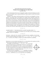
The Tate Curve C ∗ p/q d with Some of its N-torsion
C
p
!.
3 !
q. .
2
. q
.
2
. q d
. q 3
!
.
1

Definition of Modular Forms
Definition: A modular form of weight k for Γ 0 (N) is a function
which takes pairs (E, C) as input, and outputs a section of Ω ⊗k
E .
(sufficiently well-behaved, of course)

Definition of Modular Forms
Definition: A modular form of weight k for Γ 0 (N) is a function
which takes pairs (E, C) as input, and outputs a section of Ω ⊗k
E .
(sufficiently well-behaved, of course)
Definition: Suppose f is a weight k modular form for Γ 0 (N).
The q-expansion of f associated to the canonical family
(C ∗ /q d , 〈ζq〉) is the unique f (q) such that
( ) ⊗k
f (C ∗ p/q d , 〈ζq〉) = f (q) dz
z .

Definition of Modular Forms
Definition: A modular form of weight k for Γ 0 (N) is a function
which takes pairs (E, C) as input, and outputs a section of Ω ⊗k
E .
(sufficiently well-behaved, of course)
Definition: Suppose f is a weight k modular form for Γ 0 (N).
The q-expansion of f associated to the canonical family
(C ∗ /q d , 〈ζq〉) is the unique f (q) such that
( ) ⊗k
f (C ∗ p/q d , 〈ζq〉) = f (q) dz
z .
So at this point, we’ve defined q-expansions associated to
families of Tate curves, based on the moduli-theoretic definition
of modular forms. Why?

Pullbacks by Level-Lowering Maps
Suppose that Ml ∣ ∣N. It is well-known that we have maps,
π l : X 0 (N) → X 0 (M), defined by
π l (E, C) = (E/C[l], C[Ml]/C[l]).
We can also define the π l pullback of a modular form f for Γ 0 (M).

Pullbacks by Level-Lowering Maps
Suppose that Ml ∣ ∣N. It is well-known that we have maps,
π l : X 0 (N) → X 0 (M), defined by
π l (E, C) = (E/C[l], C[Ml]/C[l]).
We can also define the π l pullback of a modular form f for Γ 0 (M).
Definition: Let f be a weight k modular form for Γ 0 (M), with Ml ∣ ∣N as
above. Then we define
(π ∗ l f )(E, C) = ι ∗ (f (E/C[l], C[Ml]/C[l])),
where ι : E → E/C[l] is the canonical isogeny and
ι ∗ : Ω ⊗k
E/C[l] → Ω⊗k E .

Pullbacks by Level-Lowering Maps
Suppose that Ml ∣ ∣N. It is well-known that we have maps,
π l : X 0 (N) → X 0 (M), defined by
π l (E, C) = (E/C[l], C[Ml]/C[l]).
We can also define the π l pullback of a modular form f for Γ 0 (M).
Definition: Let f be a weight k modular form for Γ 0 (M), with Ml ∣ ∣N as
above. Then we define
(π ∗ l f )(E, C) = ι ∗ (f (E/C[l], C[Ml]/C[l])),
where ι : E → E/C[l] is the canonical isogeny and
ι ∗ : Ω ⊗k
E/C[l] → Ω⊗k E .
Big Idea: We can use Tate curve calculations to compute the
q-expansions of πl ∗ f in terms of the q-expansions of f .

Theorem 1: Suppose r, d, M, and l are positive divisors of N, such
that Ml ∣ ∣ N (so πl : X 0 (N) → X 0 (M)) and lcm(d, r) = N. Suppose ζ is
a primitive r th root of unity. Suppose f is any weight k modular form
for Γ 0 (M).

Theorem 1: Suppose r, d, M, and l are positive divisors of N, such
that Ml ∣ ∣ N (so πl : X 0 (N) → X 0 (M)) and lcm(d, r) = N. Suppose ζ is
a primitive r th root of unity. Suppose f is any weight k modular form
for Γ 0 (M).
Let g = gcd(d, N/l), and find a, b ∈ Z s.t. ad + b(N/l) = g.

Theorem 1: Suppose r, d, M, and l are positive divisors of N, such
that Ml ∣ ∣ N (so πl : X 0 (N) → X 0 (M)) and lcm(d, r) = N. Suppose ζ is
a primitive r th root of unity. Suppose f is any weight k modular form
for Γ 0 (M).
Let g = gcd(d, N/l), and find a, b ∈ Z s.t. ad + b(N/l) = g.
If
then
f (C ∗ p/(ζ bNg/d q lg2 /d ), 〈(ζq) lg/d 〉[M]) = f (q) ( )
dz ⊗k
z ,
π ∗ l f (C ∗ p/q d , 〈ζq〉) = f (q)
(
lg
d
) k ( dz
) ⊗k
z .

Theorem 1: Suppose r, d, M, and l are positive divisors of N, such
that Ml ∣ ∣ N (so πl : X 0 (N) → X 0 (M)) and lcm(d, r) = N. Suppose ζ is
a primitive r th root of unity. Suppose f is any weight k modular form
for Γ 0 (M).
Let g = gcd(d, N/l), and find a, b ∈ Z s.t. ad + b(N/l) = g.
If
then
f (C ∗ p/(ζ bNg/d q lg2 /d ), 〈(ζq) lg/d 〉[M]) = f (q) ( )
dz ⊗k
z ,
π ∗ l f (C ∗ p/q d , 〈ζq〉) = f (q)
(
lg
d
) k ( dz
) ⊗k
z .
pf/ We want to compute π ∗ l f on (C∗ p/q d , 〈ζq〉) using the definition of
π ∗ l , and in this case E = C∗ p/q d and C = 〈ζq〉. So first we apply
ι : E → E/C[l] to get C ∗ p/〈q d , (ζq) N/l 〉. Now use
C ∗ p/〈q d , (ζq) N/l 〉 ∼= −→ C ∗ p/(ζ bNg/d q lg2 /d )
z ↦→ z lg/d

Although we will only use the theorem to pull back forms of
level 1 (in particular ∆), the theorem does tell us explicitly how
to obtain the q-expansions of πl ∗ f at any cusp, given the
q-expansions at the image cusp. (It’s just a substitution, since q
is just a number here!)

Although we will only use the theorem to pull back forms of
level 1 (in particular ∆), the theorem does tell us explicitly how
to obtain the q-expansions of πl ∗ f at any cusp, given the
q-expansions at the image cusp. (It’s just a substitution, since q
is just a number here!)
Corollary 1.1: Suppose f is a form for Γ 0 (1) with q-expansion
f (q). Then the expansion at (C ∗ p/q d , 〈ζq〉) of πl ∗ f is given by
f (ζ bNg/d q lg2 /d )
(
lg
d
) k
.

Part II
Eta Products

Ligozat’s Criteria
Definition: Let ∆ be the usual weight 12 level 1 cusp form, with
q-expansion ∆(q). Let η(q) = (∆(q)) 1/24 . So
∏
∞
η(q) = q 1/24 (1 − q n ).
n=1
An eta product is an expression of the form ∏ l∣
∣ N
(η(q l )) r l.

Ligozat’s Criteria
Definition: Let ∆ be the usual weight 12 level 1 cusp form, with
q-expansion ∆(q). Let η(q) = (∆(q)) 1/24 . So
∏
∞
η(q) = q 1/24 (1 − q n ).
n=1
An eta product is an expression of the form ∏ l∣
∣ N
(η(q l )) r l.
Theorem 2: (Ligozat) An eta product is a weight 0 modular
form, i.e. a modular function, on X 0 (N), if and only if
(i) ∑ r d = 0
(ii) ∑ d · r d ≡ 0 (mod 24)
(iii) ∑ N
d · r d ≡ 0 (mod 24)
(iv) ∏ (
N
d
) rd
∈ Q 2 .

q-expansions of ∆ pullbacks
Theorem 3: For any l ∣ ∣ N, ∆(q l ) is the q-expansion at infinity of
a weight 12 modular form for Γ 0 (N). Its q-expansion associated
to the family, (C ∗ p/q d , 〈ζq〉) is given by
∆(ζ bNg/d q lg2 /d ) ( g
d
) 12 .

q-expansions of ∆ pullbacks
Theorem 3: For any l ∣ ∣ N, ∆(q l ) is the q-expansion at infinity of
a weight 12 modular form for Γ 0 (N). Its q-expansion associated
to the family, (C ∗ p/q d , 〈ζq〉) is given by
∆(ζ bNg/d q lg2 /d ) ( g
d
) 12 .
pf/ This is a direct application of Corollary 1.1. The form in
question is actually l −12 πl ∗ (∆). So from the corollary, its
expansion is
( ) 12
l −12 ∆(ζ bNg/d q lg2 /d ) lg
d .

Corollary 3.1: The leading term of the q-expansion of any
delta product (associated to a fixed family) is given by
∏
l|N
(
ζ bNg/d q lg2 /d ) r l ( g
d
) 12rl
.

Corollary 3.1: The leading term of the q-expansion of any
delta product (associated to a fixed family) is given by
∏
l|N
(
ζ bNg/d q lg2 /d ) r l ( g
d
) 12rl
.
In particular, the ord at the corresponding cusp of the
corresponding eta product is
∑
1
l·r l
24 gcd(d,N/d) d (gcd(d, N/l))2 .
l|N

Corollary 3.1: The leading term of the q-expansion of any
delta product (associated to a fixed family) is given by
∏
l|N
(
ζ bNg/d q lg2 /d ) r l ( g
d
) 12rl
.
In particular, the ord at the corresponding cusp of the
corresponding eta product is
∑
1
l·r l
24 gcd(d,N/d) d (gcd(d, N/l))2 .
l|N
Moreover, when the ord is 0 at a particular cusp, the value of
the corresponding delta product is given (up to an r th root of
unity) by
∏
( 1 d gcd(d, N/l))12r l
.
l|N

Eta products on X 0 (18)

Eta products on X 0 (18)
Applying the corollary about ords, we find:
⎡
⎤ ⎡ ⎤ ⎡
⎤
1 2 3 6 9 18 r 1 ord(d = 1)
2 1 6 3 18 9
r 2
ord(d = 2)
1 2 3 6 1 2
⎢ 2 1 6 3 2 1
·
r 3
⎥ ⎢ r 6
=
ord(d = 3)
⎥ ⎢ ord(d = 6)
⎥
⎣ 9 18 3 6 1 2 ⎦ ⎣ r 9
⎦ ⎣ ord(d = 9) ⎦
18 9 6 3 2 1 r 18 ord(d = 18)
Note: There are two cusps with d = 3 and two with d = 6.

Eta products on X 0 (18)
Applying the corollary about ords, we find:
⎡
⎤ ⎡ ⎤ ⎡
⎤
1 2 3 6 9 18 r 1 ord(d = 1)
2 1 6 3 18 9
r 2
ord(d = 2)
1 2 3 6 1 2
⎢ 2 1 6 3 2 1
·
r 3
⎥ ⎢ r 6
=
ord(d = 3)
⎥ ⎢ ord(d = 6)
⎥
⎣ 9 18 3 6 1 2 ⎦ ⎣ r 9
⎦ ⎣ ord(d = 9) ⎦
18 9 6 3 2 1 r 18 ord(d = 18)
Note: There are two cusps with d = 3 and two with d = 6.
Let f = η2 2 η 9
η 1 η 2 18
.
By Ligozat, it is a legitimate function, and by above it has divisor
(1/2) − (∞). Hence it is a parameter on this genus 0 curve.

Moreover, the values of f 24 at the d = 18, 6, 3, and 2 cusps are
3 24 , 3 12 , 3 12 , and 1 (respectively, up to a root of unity). These
values can be easily verified (in this case) by choosing eta
products which vanish at the other cusps, and then comparing
with f .

Moreover, the values of f 24 at the d = 18, 6, 3, and 2 cusps are
3 24 , 3 12 , 3 12 , and 1 (respectively, up to a root of unity). These
values can be easily verified (in this case) by choosing eta
products which vanish at the other cusps, and then comparing
with f .
x = η2 1 η 6η 9
η 2 η 3 η 2 18
(x) = (0) − (∞) x = f − 3

Moreover, the values of f 24 at the d = 18, 6, 3, and 2 cusps are
3 24 , 3 12 , 3 12 , and 1 (respectively, up to a root of unity). These
values can be easily verified (in this case) by choosing eta
products which vanish at the other cusps, and then comparing
with f .
x = η2 1 η 6η 9
η 2 η 3 η 2 18
(x) = (0) − (∞) x = f − 3
y = η 2η 6 3
η 2 1 η2 6 η3 18
(y) = c 6,1 + c 6,2 − 2(∞) y = f 2 + 3

Moreover, the values of f 24 at the d = 18, 6, 3, and 2 cusps are
3 24 , 3 12 , 3 12 , and 1 (respectively, up to a root of unity). These
values can be easily verified (in this case) by choosing eta
products which vanish at the other cusps, and then comparing
with f .
x = η2 1 η 6η 9
η 2 η 3 η 2 18
(x) = (0) − (∞) x = f − 3
y = η 2η 6 3
η 2 1 η2 6 η3 18
(y) = c 6,1 + c 6,2 − 2(∞) y = f 2 + 3
z = η 1η 8 6 η3 9
η 2 2 η4 3 η6 18
(z) = c 3,1 + c 3,2 − 2(∞) z = f 2 − 3f + 3

Moreover, the values of f 24 at the d = 18, 6, 3, and 2 cusps are
3 24 , 3 12 , 3 12 , and 1 (respectively, up to a root of unity). These
values can be easily verified (in this case) by choosing eta
products which vanish at the other cusps, and then comparing
with f .
x = η2 1 η 6η 9
η 2 η 3 η 2 18
(x) = (0) − (∞) x = f − 3
y = η 2η 6 3
η 2 1 η2 6 η3 18
(y) = c 6,1 + c 6,2 − 2(∞) y = f 2 + 3
z = η 1η 8 6 η3 9
η 2 2 η4 3 η6 18
(z) = c 3,1 + c 3,2 − 2(∞) z = f 2 − 3f + 3
w = η 6η 3 9
η 3 η 3 18
(w) = (1/9) − (∞) w = f − 1

What if there aren’t enough eta products?

What if there aren’t enough eta products?
Answer: There are. Philosophically, Ligozat works in different
weights, and we can apply the θ operator. Weight 0 to weight 2
(functions to differentials) is especially straightforward.

What if there aren’t enough eta products?
Answer: There are. Philosophically, Ligozat works in different
weights, and we can apply the θ operator. Weight 0 to weight 2
(functions to differentials) is especially straightforward.
Theorem 4: (Shimura) Let f be a form of even weight k. Let
ν = f (z)(dz) k/2 . Then
(∑ )
Div(f ) = Div(ν) + (k/2) · (1 − e
−1
i
)P i + cusps ,
where {P i } are the elliptic points of order e i .

A Nice Example Involving X 0 (11)
Doing the usual thing, we find that t = η1 12/η12
11
is a legitimate
function with divisor 5(0) − 5(∞). We also get a weight two
cusp form by taking (η 1 η 11 ) 2 . Using the preceding theorem, its
divisor (as a form) is (0) + (∞).

A Nice Example Involving X 0 (11)
Doing the usual thing, we find that t = η1 12/η12
11
is a legitimate
function with divisor 5(0) − 5(∞). We also get a weight two
cusp form by taking (η 1 η 11 ) 2 . Using the preceding theorem, its
divisor (as a form) is (0) + (∞).
There aren’t any elliptic points. So the function,
x :=
dt/t
(η 1 η 11 ) 2 ,
has degree 2, with a simple pole at each cusp. This implies that
x is a parameter on X 0 (11) + := X 0 (11)/w 11 . By comparing
q-expansions, we find:
t 2 + 1 5 5 (x 5 +170x 4 +9345x 3 +167320x 2 −7903458)t +11 6 = 0.

Remark:
This reduces mod 11 to
t 2 + (x − 2) 2 (x + 3) 3 t = 0.
It’s the blow-down of the Deligne-Rapoport model!!

Remark:
This reduces mod 11 to
t 2 + (x − 2) 2 (x + 3) 3 t = 0.
It’s the blow-down of the Deligne-Rapoport model!!
By letting
y = 2 · 55 t + (x 5 + 170x 4 + 9345x 3 + 167320x 2 − 7903458)
(x + 47)(x 2 + 89x + 1424)
we arrive at the “nicer” model:
y 2 = (x − 8)(x 3 + 76x 2 − 8x + 188).

Remark:
This reduces mod 11 to
t 2 + (x − 2) 2 (x + 3) 3 t = 0.
It’s the blow-down of the Deligne-Rapoport model!!
By letting
y = 2 · 55 t + (x 5 + 170x 4 + 9345x 3 + 167320x 2 − 7903458)
(x + 47)(x 2 + 89x + 1424)
we arrive at the “nicer” model:
y 2 = (x − 8)(x 3 + 76x 2 − 8x + 188).
Note: π1 ∗ j = (60y + 61x 2 + 864x − 2016) 3
5 6 .
t

Conclusions:

Conclusions:
(1) It’s fairly straightforward to compute the q-expansion of the
pullback of a modular form for Γ 0 (N) via πl ∗ in terms of the
expansion at the appropriate image cusp.

Conclusions:
(1) It’s fairly straightforward to compute the q-expansion of the
pullback of a modular form for Γ 0 (N) via πl ∗ in terms of the
expansion at the appropriate image cusp.
(2) Using (1), we have nice formulas for everything you’d want
to know about eta products.

Conclusions:
(1) It’s fairly straightforward to compute the q-expansion of the
pullback of a modular form for Γ 0 (N) via πl ∗ in terms of the
expansion at the appropriate image cusp.
(2) Using (1), we have nice formulas for everything you’d want
to know about eta products.
(3) Eta products can be used to get really nice explicit models
for X 0 (N), even if N = p.

Part III
Implementation

Eta Product Package Wish List
Easy: (just derived the formulas)

Eta Product Package Wish List
Easy: (just derived the formulas)
(1) Ligozat check
(2) Matrix that converts exponent lists to cuspidal divisors
(3) Value of delta product at any cusp not in the support

Eta Product Package Wish List
Easy: (just derived the formulas)
(1) Ligozat check
(2) Matrix that converts exponent lists to cuspidal divisors
(3) Value of delta product at any cusp not in the support
Slightly Harder: (just a pain)

Eta Product Package Wish List
Easy: (just derived the formulas)
(1) Ligozat check
(2) Matrix that converts exponent lists to cuspidal divisors
(3) Value of delta product at any cusp not in the support
Slightly Harder: (just a pain)
(4) Basis for eta products (as a Z-module).
(5) Eta products of minimal degree.
(6) Equations relating choice of finitely many eta products.

Basis Calculation for X 0 (18)
Ligozat condition is equivalent to a system of (2 + p(N))
homogeneous linear congruences mod 24, in (d(N) − 1)
variables (where p(N) is the number of primes dividing N).
Simple Gaussian elimination should give a basis over Z/24Z
and then over Z.

Basis Calculation for X 0 (18)
Ligozat condition is equivalent to a system of (2 + p(N))
homogeneous linear congruences mod 24, in (d(N) − 1)
variables (where p(N) is the number of primes dividing N).
Simple Gaussian elimination should give a basis over Z/24Z
and then over Z.
r 1 +2r 2 +3r 3 +6r 6 +9r 9 +18r 18 ≡ 0 (mod 24)
18r 1 +9r 2 +6r 3 +3r 6 +2r 9 +r 18 ≡ 0 (mod 24)
12r 1 +12r 3 +12r 9 ≡ 0 (mod 24)
12r 3 +12r 6 ≡ 0 (mod 24)

Basis Calculation for X 0 (18)
Ligozat condition is equivalent to a system of (2 + p(N))
homogeneous linear congruences mod 24, in (d(N) − 1)
variables (where p(N) is the number of primes dividing N).
Simple Gaussian elimination should give a basis over Z/24Z
and then over Z.
r 1 +2r 2 +3r 3 +6r 6 +9r 9 +18r 18 ≡ 0 (mod 24)
18r 1 +9r 2 +6r 3 +3r 6 +2r 9 +r 18 ≡ 0 (mod 24)
12r 1 +12r 3 +12r 9 ≡ 0 (mod 24)
12r 3
⎡
+12r 6 ≡ 0
⎤
(mod 24)
−17 −16 −15 −12 −9
17 8 5 2 1 ⎥
12 0 12 0 12⎦
0 0 12 12 0
⎢
⎣

Basis Calculation for X 0 (18)
Ligozat condition is equivalent to a system of (2 + p(N))
homogeneous linear congruences mod 24, in (d(N) − 1)
variables (where p(N) is the number of primes dividing N).
Simple Gaussian elimination should give a basis over Z/24Z
and then over Z.
r 1 +2r 2 +3r 3 +6r 6 +9r 9 +18r 18 ≡ 0 (mod 24)
18r 1 +9r 2 +6r 3 +3r 6 +2r 9 +r 18 ≡ 0 (mod 24)
12r 1 +12r 3 +12r 9 ≡ 0 (mod 24)
12r 3 +12r 6 ≡ 0 (mod 24)
⎡
⎤
−17 −16 −15 −12 −9
⎢ 17 8 5 2 1 ⎥
⎣ 12 0 12 0 12⎦
0 0 12 12 0
⎡ ⎤ ⎡ ⎤ ⎡ ⎤ ⎡ ⎤ ⎡ ⎤
r 1 0 4 3 −1
r 2
3
−2
0
−1
r 3
⎢ r
⎣ 6 ⎥
⎦ = a 0
⎢ 0 ⎥
⎣ ⎦ + b 4
⎢ 0 ⎥
⎣ ⎦ + c −1
⎢ 1 ⎥
⎣ ⎦ + d 0
⎢ 0 ⎥
⎣ ⎦
r 9 0 0 0 1
r 18 −3 −6 −3 1

Using eta products to find an equation on X 0 (26)

Using eta products to find an equation on X 0 (26)
On X 0 (26), the eta product divisor matrix is:
⎡
⎤ ⎡ ⎤ ⎡
1 2 13 26 r 1
⎢ 2 1 26 13
⎥
⎣13 26 1 2 ⎦ ·
⎢ r 2
⎥
⎣r 13
⎦ = ⎢
⎣
26 13 2 1 r 26
Note: Only one cusp of each width this time.
ord(d = 1)
ord(d = 2)
ord(d = 13)
ord(d = 26)
⎤
⎥
⎦

Using eta products to find an equation on X 0 (26)
On X 0 (26), the eta product divisor matrix is:
⎡
⎤ ⎡ ⎤ ⎡
1 2 13 26 r 1
⎢ 2 1 26 13
⎥
⎣13 26 1 2 ⎦ ·
⎢ r 2
⎥
⎣r 13
⎦ = ⎢
⎣
26 13 2 1 r 26
Note: Only one cusp of each width this time.
ord(d = 1)
ord(d = 2)
ord(d = 13)
ord(d = 26)
Initially, we choose the following two eta products:
⎤
⎥
⎦
t = η2 2 η2 13
η 2 26 η2 1
u = η4 2 η2 13
η 4 26 η2 1
(t) = (1/2) + (1/13) − (0) − (∞)
(u) = 3(1/2) − 3(∞)

Since u = 13 at the cusp 0, we let v = t(u − 13) and must have:
a 1 u 4 + a 2 v 3 + a 3 v 2 u + a 4 vu 2 + a 5 u 3 +
a 6 v 2 + a 7 uv + a 8 u 2 + a 9 v + a 10 u + a 11 = 0.
By comparing q-expansions, we find:
u 4 − v 3 + 4uv 2 + 4u 2 v − 27u 3 − 52uv + 195u 2 − 169u = 0.

Since u = 13 at the cusp 0, we let v = t(u − 13) and must have:
a 1 u 4 + a 2 v 3 + a 3 v 2 u + a 4 vu 2 + a 5 u 3 +
a 6 v 2 + a 7 uv + a 8 u 2 + a 9 v + a 10 u + a 11 = 0.
By comparing q-expansions, we find:
u 4 − v 3 + 4uv 2 + 4u 2 v − 27u 3 − 52uv + 195u 2 − 169u = 0.
Changing back to (t, u), we have:
u 2 − t 3 u + 4t 2 u + 4tu − u + 13t 3 = 0.

Since u = 13 at the cusp 0, we let v = t(u − 13) and must have:
a 1 u 4 + a 2 v 3 + a 3 v 2 u + a 4 vu 2 + a 5 u 3 +
a 6 v 2 + a 7 uv + a 8 u 2 + a 9 v + a 10 u + a 11 = 0.
By comparing q-expansions, we find:
u 4 − v 3 + 4uv 2 + 4u 2 v − 27u 3 − 52uv + 195u 2 − 169u = 0.
Changing back to (t, u), we have:
u 2 − t 3 u + 4t 2 u + 4tu − u + 13t 3 = 0.
Finally, with x = t and y = 2u − t 3 + 4t 2 + 4t − 1 we arrive at:
y 2 = x 6 − 8x 5 + 8x 4 − 18x 3 + 8x 2 − 8x + 1.

Since u = 13 at the cusp 0, we let v = t(u − 13) and must have:
a 1 u 4 + a 2 v 3 + a 3 v 2 u + a 4 vu 2 + a 5 u 3 +
a 6 v 2 + a 7 uv + a 8 u 2 + a 9 v + a 10 u + a 11 = 0.
By comparing q-expansions, we find:
u 4 − v 3 + 4uv 2 + 4u 2 v − 27u 3 − 52uv + 195u 2 − 169u = 0.
Changing back to (t, u), we have:
u 2 − t 3 u + 4t 2 u + 4tu − u + 13t 3 = 0.
Finally, with x = t and y = 2u − t 3 + 4t 2 + 4t − 1 we arrive at:
y 2 = x 6 − 8x 5 + 8x 4 − 18x 3 + 8x 2 − 8x + 1.
Remark: π1 ∗(η2 1 /η2 13 ) = u/t2 and π2 ∗(η2 1 /η2 13 ) = u/t.