Biol 529 Plant Ecology Similarity among communities Communities ...

Biol 529 Plant Ecology
Similarity among communities
Communities can differ in a number of ways. Considering only the plant component of a system, two
communities can differ in species composition (taxonomy), total number of species (richness), and the
relative abundance of species (evenness). Species diversity refers to a community-­‐level concept that
combines both richness and evenness.
We use a number of different indices to estimate the similarity of two communities. Considerable
controversy exists about the effectiveness of these indices as they vary in performance for things like total
number of species involved, influence of rare species, etc. A number of papers recently have explored what
an appropriate index might be.
We will use a few of the common ones that you will frequently come across in the literature so you can get an
impression of their usefulness. They fall into two categories, presence-­‐absence measures, which focus on
richness and composition, and abundance measures, with incorporate richness, composition, and abundance.
We will use the following indices:
Jaccard (presence-­‐absence)
S J =
a/a+b+c
Sorensen-Dice (Sorensen or Sorensen binary) (presence-­‐absence)
S SD =
2a/2a+b+c
Bray-Curtis (sometimes called Pielou’s percentage similarity or Czekanowski’s)
Where:
S BC = ∑ 2*min(n 1i, n 2i)
∑n 1i+∑n 2i
a=number of species in both sites
b= number of species in second site only
c= number of species in first site only
n 1i = the number of individuals or % cover or Importance value of the ith species in sample 1
n 2i = the number of individuals or % cover or Importance value of the ith species in sample 2
min=refers to the lower abundance value for the species of the two samples being compared
The Jaccard index, also known as the Jaccard similarity coefficient (originally coined coefficient de communauté
by Paul Jaccard), is a statistic used for comparing the similarity and diversity of sample sets. The Jaccard coefficient
measures similarity between sample sets, and is defined as the size of the intersection divided by the size of the
union of the sample sets. This index only uses presence-absence data.
The Sørensen index, also known as Sørensen’s similarity coefficient, is a statistic used for comparing the
similarity of two samples. It was developed by the botanist Thorvald Sørensen and published in 1948. It also uses
on presence-absence data. When you use both the Jaccard and Sorensen Index on the same data set, note how they
differ in performance.
Sorensen’s Index is easily extended to abundance instead of incidence of species. This quantitative version of the
Sørensen index is also known as the Bray-Curtis Similarity index. When using the Bray-­‐Curtis quantitative

index, the “minimum” value (# individuals or %cover or Importance Value) for a species when comparing two
samples is used for the numerator values.
Ecologists often use different names to describe the same index. For example, Pielou’s percentage
similarity is the same as Bray-­‐Curtis, Sorensen’s quantitative index and the Czekanowski’s quantitative
index (but there is disagreement about this latter case).
Lab Problems:
We will use a made-­‐up data set to compare the performance of these similarity indices. Imagine comparing
two communities (samples) with 30 species each and 25 species are found in both samples. Run your
calculations. Then modify the proportions in the two samples so you can understand how the indices
perform. Change the proportions so both samples keep 30 species, but only 20 are in common, then 15, then
10, then 5. Then contrast a 30 species community with a 20 species community (start with 20 species in
common), and make similar proportion shifts.
Now let’s see how the total number of species influences things. Start with comparing a two communities of
30 species with 20 species in common (you did this above). Now change it so they both have 30 species, but
only 19 in common. Now compare two communities of 15 species each with 10 species in common, and then
with 9 species in common. Finally, compare two communities of 3 species each, with 2 species in common,
then change it to 1 species in common. In this second round, we’re only shifting 1 species each time, but
because of ‘proportion’ shifts, the measures perform quite differently. If we were using Bray-­‐Curtis values,
the shifts may not have changed in the same manner.
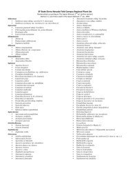
Assignment: Take the Sierran data and calculate similarities between one elevation and that above or below
it.
1. Create an ‘average IV matrix’ for each species for each elevation.
2. Create a presence-­‐absence matrix as well.
3. Calculate a Jaccard Index for 7000 & 6500, 6500 & 6000, 6000 & 5500, etc. Do the same for Sorensen’s and
Bray-­‐Curtis Index.
4. Create a graph for each index. Plot the Index value on the Y-­‐axis. For the X-­‐axis, use the ‘joint’ elevation
value.
5. Examine the graphs. In a paragraph or two, discuss whether these similarity indices suggest whether
there are one, two, three or more plant communities along the elevation gradient. In other words, is there a
significant change in the value of the indices such that one elevation is much more different (less similar) to
the next elevation than is typical for the other elevation pairs?
6. You can work in groups to do the calculations and discuss them, but write the paragraph by yourself.
7. Turn in the graphs you make along with the discussion.