Quaternions and Rotations∗ - Iowa State University

Quaternions and Rotations ∗
(Com S 477/577 Notes)
Yan-Bin Jia
Sep 20, 2010
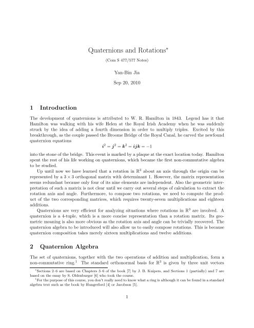
1 Introduction
The development of quaternions is attributed to W. R. Hamilton in 1843. Legend has it that
Hamilton was walking with his wife Helen at the Royal Irish Academy when he was suddenly
struck by the idea of adding a fourth dimension in order to multiply triples. Excited by this
breakthrough, as the couple passed the Broome Bridge of the Royal Canal, he carved the newfound
quaternion equations
i 2 = j 2 = k 2 = ijk = −1
into the stone of the bridge. This event is marked by a plaque at the exact location today. Hamilton
spent the rest of his life working on quaternions, which became the first non-commutative algebra
to be studied.
Up until now we have learned that a rotation in R 3 about an axis through the origin can be
represented by a 3 × 3 orthogonal matrix with determinant 1. However, the matrix representation
seems redundant because only four of its nine elements are independent. Also the geometric interpretation
of such a matrix is not clear until we carry out several steps of calculation to extract the
rotation axis and angle. Furthermore, to compose two rotations, we need to compute the product
of the two corresponding matrices, which requires twenty-seven multiplications and eighteen
additions.
Quaternions are very efficient for analyzing situations where rotations in R 3 are involved. A
quaternion is a 4-tuple, which is a more concise representation than a rotation matrix. Its geometric
meaning is also more obvious as the rotation axis and angle can be trivially recovered. The
quaternion algebra to be introduced will also allow us to easily compose rotations. This is because
quaternion composition takes merely sixteen multiplications and twelve additions.
2 Quaternion Algebra
The set of quaternions, together with the two operations of addition and multiplication, form a
non-commutative ring. 1 The standard orthonormal basis for R 3 is given by three unit vectors
∗ Sections 2–6 are based on Chapters 3–6 of the book [7] by J. B. Kuipers, and Sections 1 (partially) and 7 are
based on the essay by S. Oldenburger [6] who took the course.
1 For the purpose of this course, you don’t really need to know what a ring is although it can be found in a standard
algebra text such as the book by Hungerford [4] or Jacobson [5].
1

i = (1,0,0), j = (0,1,0), k = (0,0,1). A quaternion q is defined as the sum of a scalar q 0 and a
vector q = (q 1 ,q 2 ,q 3 ); namely,
2.1 Addition and Multiplication
q = q 0 + q = q 0 + q 1 i + q 2 j + q 3 k.
Addition of two quaternions acts componentwise. More specifically, consider the quaternion q above
and another quaternion
p = p 0 + p 1 i + p 2 j + p 3 k.
Then we have
p + q = (p 0 + q 0 ) + (p 1 + q 1 )i + (p 2 + q 2 )j + (p 3 + q 3 )k.
Every quaternion q has a negative −q with components −q i , i = 0,1,2,3.
The product of two quaternions satisfies these fundamental rules introduced by Hamilton:
i 2 = j 2 = k 2 = ijk = −1,
ij = k = −ji,
jk = i = −kj,
ki = j = −ik.
Now we can give the product of two quaternions p and q:
pq = (p 0 + p 1 i + p 2 j + p 3 k)(q 0 + q 1 i + q 2 j + q 3 k)
= p 0 q 0 − (p 1 q 1 + p 2 q 2 + p 3 q 3 ) + p 0 (q 1 i + q 2 j + q 3 k) + q 0 (p 1 i + p 2 j + p 3 k)
+(p 2 q 3 − p 3 q 2 )i + (p 3 q 1 − p 1 q 3 )j + (p 1 q 2 − p 2 q 1 )k.
Whew! It is too long to remember or even to understand what is going on. Fortunately, we can
utilize the inner product and cross product of two vectors in R 3 to write the above quaternion
product in a more concise form:
pq = p 0 q 0 − p · q + p 0 q + q 0 p + p × q. (1)
In the above, p = (p 1 ,p 2 ,p 3 ) and q = (q 1 ,q 2 ,q 3 ) are the vector parts of p and q, respectively.
Example 1. Suppose the two vectors are given as follows:
p = 3 + i − 2j + k,
q = 2 − i + 2j + 3k.
We single out their vector parts p = (1, −2, 1) and q = (−1, 2, 3) and calculate their inner and cross products:
p · q = −2,
i j k
p × q =
1 −2 1
∣ −1 2 3 ∣
= −8i − 4j.
2

By (1) the quaternion product is then
pq = 6 − (−2) + 3(−i + 2j + 3k) + 2(i − 2j + k) + (−8i − 4j)
= 8 − 9i − 2j + 11k.
We see that the product of two quaternions is still a quaternion with scalar part p 0 q 0 −p·q and
vector part p 0 q + q 0 p + p × q. The set of quaternions is closed under multiplication and addition.
It is not difficult to verify that multiplication of quaternions is distributive over addition. The
identity quaternion has real part 1 and vector part 0.
2.2 Complex Conjugate, Norm, and Inverse
Let q = q 0 + q = q 0 + q 1 i + q 2 j + q 3 k be a quaternion. The complex conjugate of q, denoted q ∗ , is
defined as
q ∗ = q 0 − q = q 0 − q 1 i − q 2 j − q 3 k.
From the definition we immediately have
(q ∗ ) ∗ = q 0 − (−q) = q,
q + q ∗ = 2q 0 ,
q ∗ q = (q 0 − q)(q 0 + q)
= q 0 q 0 − (−q) · q + q 0 q + (−q)q 0 + (−q) × q by (1)
= q 2 0 + q · q
= q 2 0 + q2 1 + q2 2 + q2 3
= qq ∗ .
Given two quaternions p and q, we can easily verify that
(pq) ∗ = q ∗ p ∗ . (2)
The norm of a quaternion q, denoted by |q|, is the scalar |q| = √ q ∗ q. A quaternion is called a
unit quaternion if its norm is 1. The norm of the product of two quaternions p and q is the product
of the individual norms, for we have
|pq| 2
= (pq)(pq) ∗
= pqq ∗ p ∗
= p|q| 2 p ∗
= pp ∗ |q| 2
= |p| 2 |q| 2 .
The inverse of a quaternion q is defined as
q −1 = q∗
|q| 2.
We can easily verify that q −1 q = qq −1 = 1. In the case q is a unit quaternion, the inverse is its
conjugate q ∗ .
3

3 Quaternion Rotation Operator
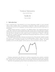
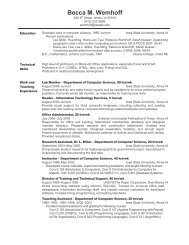
How can a quaternion, which lives in R 4 , operate on a vector, which lives in R 3 ? First, we note
that a vector v ∈ R 3 is a pure quaternion whose real part is zero. Let us consider a unit quaternion
q = q 0 + q only. That q 2 0 + ‖q‖2 = 1 implies that there must exist some angle θ such that
cos 2 θ = q 2 0 ,
sin 2 θ = ‖q‖ 2 .
In fact, there exists a unique θ ∈ [0,π] such that cos θ = q 0 and sin θ = ‖q‖. The unit quaternion
can now be written in terms of the angle θ and the unit vector u = q/‖q‖:
q = cos θ + usin θ.
Pure Quaternions
R
3
v
v = 0 + v
R
4
Quaternions
Using the unit quaternion q we define an operator on vectors v ∈ R 3 :
L q (v) = qvq ∗
= (q 2 0 − ‖q‖ 2 )v + 2(q · v)q + 2q 0 (q × v). (3)
Here we make two observations. First, the quaternion operator (3) does not change the length of
the vector v for
‖L q (v)‖
= ‖qvq ∗ ‖
= |q| · ‖v‖ · |q ∗ |
= ‖v‖.
Second, the direction of v, if along q, is left unchanged by the operator L q . To verify this, we let
v = kq and have
qvq ∗
= q(kq)q ∗
= (q0 2 − ‖q‖ 2 )(kq) + 2(q · kq)q + 2q 0 (q × kq)
= k(q0 2 + ‖q‖2 )q
= kq.
The two observations make us guess that the operator L q acts like a rotation about q. This is made
precise by the next theorem.
Before proceeding with the theorem, we remark that the operator L q is linear over R 3 . For any
two vectors v 1 ,v 2 ∈ R 3 and any a 1 ,a 2 ∈ R we can show that
L q (a 1 v 1 + a 2 v 2 ) = a 1 L q (v 1 ) + a 2 L q (v 2 ).
4

Theorem 1 For any unit quaternion
and for any vector v ∈ R 3 the action of the operator
q = q 0 + q = cos θ 2 + u sin θ 2 , (4)
L q (v) = qvq ∗
on v is equivalent to a rotation of the vector through an angle θ about u as the axis of rotation.
Proof Given a vector v ∈ R 3 , we decompose it as v = a + n, where a is the component along
the vector q and n is the component normal to q. Then we show that under the operator L q , a is
invariant, while n is rotated about q through an angle θ. Since the operator is linear, this shows
that the image qvq ∗ is indeed interpreted as a rotation of v about q through an angle θ.
We know from an early reasoning that a is invariant under L q . So let us focus on the effect of
L q on the orthogonal component n. We have
L q (n) = (q 2 0 − ‖q‖2 )n + 2(q · n)q + 2q 0 (q × n)
= (q 2 0 − ‖q‖2 )n + 2q 0 (q × n)
= (q 2 0 − ‖q‖2 )n + 2q 0 ‖q‖(u × n),
where in the last step above we introduced u = q/‖q‖. Denote n ⊥ = u × n. So the last equation
becomes
L q (n) = (q 2 0 − ‖q‖ 2 )n + 2q 0 ‖q‖n ⊥ . (5)
Note that n ⊥ and n have the same length:
‖n ⊥ ‖ = ‖n × u‖ = ‖n‖ · ‖u‖sin π 2 = ‖n‖.
Finally, we rewrite (5) into the form
(
L q (n) = cos 2 θ 2 − θ ) (
sin2 n + 2cos θ 2 2 sin θ )
n ⊥
2
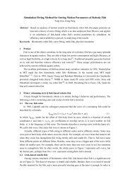
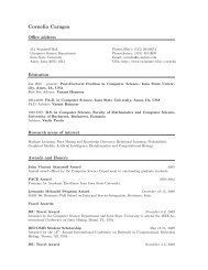
= cos θn + sin θn ⊥ .
Namely, the resulting vector is a rotation of n through an angle θ in the plane defined by n and
n ⊥ . See the figure below. This vector is clearly orthogonal to the rotation axis.
n
L q ( n)
θ
q
n
5

We substitute the unit quaternion form (4) into (3) to obtain the resulting vector from rotating
a vector v about the axis u through θ:
(
L p (v) = cos 2 θ 2 − θ )
sin2 v + 2
(usin θ )
2 2 · v usin θ 2 + 2cos θ (usin θ )
2 2 × v
= cos θ · v + (1 − cos θ)(u · v)u + sinθ · (u × v). (6)
Example 2. Consider a rotation about an axis defined by (1, 1, 1) through an angle of 2π/3. About this
axis, the basis vectors i, j, and k generate the same cone when rotated through 2π. We define a unit vector
u = 1 √
3
(1, 1, 1).
Let the rotation angle θ = 2π/3. The quaternion q defines the rotation is then given as
v = − 1 ⎝ 1 0 ⎠ +
2
0
⎛
− 1 ⎞ ⎛
2
= ⎝ 0 ⎠ ⎜
+ ⎝
0
q = cos θ 2 + usin θ 2
= 1 2 + 1 2 i + 1 2 j + 1 2 k.
Let us compute the effect of rotation on the basis vector i = (1, 0, 0). We obtain the resulting vector
using (6):
⎛ ⎞
⎛
(
1 + 1 )
1 1
· √ · √ ⎝ 1 ⎞ ⎛
√
1 ⎠ 3
+
2 3 3 2 · 1
√ ⎝ 1 ⎞ ⎛
1 ⎠ × ⎝ 1 ⎞
0 ⎠
1 3 1 0
⎞ ⎛ ⎞
= j.
1
2
1
2
1
2
⎟ ⎜
⎠ + ⎝
0
1
2
− 1 2
⎟
⎠
The rotation of v under the operator L q can also be interpreted from the perspective of an
observer attached to the vector v. What he sees happening is that the coordinate frame rotates
through the angle −θ about the same axis defined by the quaternion.
Theorem 2 For any unit quaternion
q = q 0 + q = cos θ 2 + u sin θ 2 ,
and for any vector v ∈ R 3 the action of the operator
L q ∗(v) = q ∗ v(q ∗ ) ∗ = q ∗ vq
is a rotation of the coordinate frame about the axis u through an angle θ while v is not rotated.
Equivalently, the operator L q ∗ rotates the vector v with respect to the coordinate frame through
an angle −θ about q.
The quaternion operator L q (v) = qvq ∗ may be interpreted as a point or vector rotation with
respect to the (fixed) coordinate frame. The quaternion operator L q ∗(v) = q ∗ vq may be interpreted
as a coordinate frame rotation with respect to the (fixed) space of points.
6

4 Quaternion Operator Sequences
Let p and q be two unit quaternions. We first apply the operator L p to the vector u and obtain
the vector v. To v we then apply the operator L q and obtain the vector w. Equivalently, we apply
the composition L q ◦ L p of the two operators:
w = L q (v)
= qvq ∗
= q(pup ∗ )q ∗
= (qp)u(qp) ∗
= L qp (u).
Because p and q are unit quaternions, so is the product qp. Hence the above equation describes a
rotation operator whose defining quaternion is the product of the two quaternions p and q. The
axis and angle of the composite rotation is given by the product qp.
Similarly, consider the quaternion operators L p ∗(u) = p ∗ up and L q ∗(v) = q ∗ vq which carry
out rotations of the coordinate system determined by quaternions p and q, respectively. Then the
quaternion product pq defines an operator L (pq) ∗, which represents a sequence of operators L p ∗
followed by L q ∗. The axis and angle of rotation of L (pq) ∗ are those represented by the quaternion
product pq.
Example 3. We now use the quaternion method to find the axis and angle of the composite rotation in
the Satellite tracking example from the notes titled “Space Rotations”. Recall that the tracking application
takes a rotation about the z-axis through a bearing angle α followed by a rotation about the new y-axis
through an elevation angle β. After these two rotations, the new x-axis points toward the satellite. The two
rotations are respectively described by the two quaternions below:
p = cos α 2 + sin α 2 k,
q = cos β 2 + sin β 2 j.
Since we are rotating the coordinate frame, the two operators L p ∗ and L q ∗ are applied sequentially. The
composite rotation operator is L (pq) ∗, which transforms coordinates in the station frame to those in the
tracking frame. And the quaternion describing the composition rotation is the product pq which is as
follows.
pq =
(cos α 2 + sin α ) (
2 k cos β 2 + sin β )
2 j
= cos α 2 cos β 2 + cos α 2 sin β 2 j + sin α 2 cos β 2 k + sin α 2 sin β (k × j)
2
= cos α 2 cos β 2 − sin α 2 sin β 2 i + cos α 2 sin β 2 j + sin α 2 cos β 2 k.
The axis of the composite rotation is defined by the vector
(
v = − sin α 2 sin β 2 , cos α 2 sin β 2 , sin α 2 cos β )
. (7)
2
And the angle of rotation θ satisfies
cos θ 2
sin θ 2
= cos α 2 cos β 2 ,
= ‖v‖.
7

The cosine is same as obtained in Section 3 of the handouts titled “Rotation in the Space” for we have
cosθ = 2 cos 2 θ 2 − 1
= 2 cos 2 α 2 cos2 β 2 − 1
= 2 cosα + 1 · cosβ + 1 − 1
2 2
cosα cosβ + cosα + cosβ − 1
= .
2
Note that the rotation axis and angle in that section transforms coordinates in the tracking frame to those
in the station frame. This explains why the axis v in (7) is opposite to the one obtained in that section
while the angle is the same.
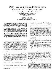
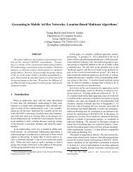
5 Application: 3-D Shape Registration
An important problem in model-based recognition is to find the transformation of a set of data
points that yields the best match of these points against a shape model. The process is often
referred to as data registration. The data points are typically measured on a real object by range
sensors, touch sensors, etc., and given in Cartesian coordinates. The quality of a match is often
described as the total squared distance from the data points to the model. When multiple shape
models are possible, the one that results in the least total distance is then recognized as the shape
of the object.
Quaternions are very effective in solving the above least-squares-based registration problem. Let
us begin with a formulation of the problem in 3D. Let {p 1 ,p 2 ,... ,p n } be a set of data points. We
assume that p 1 ,... ,p n are to be matched against the points q 1 ,... ,q n on a shape model. Namely,
the correspondences between the data points and those on the model have been predetermined.
Then the problem is to find a rotation, represented by an orthogonal matrix R with det(R) = 1,
and a translation b as the solution to the following minimization:
min
R,b
n∑
‖Rp i + b − q i ‖ 2 . (8)
i=1
q 1
q 5
q 3
p 1
p 5
p 3
p 2
rotation
translation
q 4
q 7
p 7
q 6
q 2
p 4
p 6
Data
Model
8

We begin by computing the centroids of the two sets of points:
¯p =
1 n
¯q =
1 n
n∑
p i ;
i=1
n∑
q i .
The relative coordinates of all the points to their centroids are obtained as, for 1 ≤ i ≤ n,
i=1
p ′ i
q ′ i
= p i − ¯p;
= q i − ¯q.
Clearly, we have
n∑
p ′ i =
i=1
n∑
q ′ i =
i=1
n∑
p i − n¯p =
i=1
n∑
q i − n¯q =
i=1
n∑
i=1
n∑
i=1
p i − n · 1
n
q i − n · 1
n
n∑
p i = 0; (9)
i=1
n∑
q i = 0. (10)
i=1
Let us rewrite the objective function in (8) in terms of ¯p, ¯q,p ′ i ,q′ i :
n∑
‖Rp i + b − q i ‖ 2 =
i=1
=
=
=
=
n∑
‖Rp ′ i − q′ i + R¯p − ¯q + b‖2
i=1
n∑
(Rp ′ i − q′ i + R¯p − ¯q + b) · (Rp′ i − q′ i + R¯p − ¯q + b)
i=1
(
n∑
‖Rp ′ i − q ′ i‖ 2 + 2
i=1
)
n∑
(Rp ′ i − q ′ i) · (R¯p − ¯q + b) + n‖R¯p − ¯q + b‖ 2
i=1
(
n∑
‖Rp ′ i − q ′ i‖ 2 + 2 R
i=1
n∑
p ′ i −
i=1
n∑
i=1
q ′ i
)
· (R¯p − ¯q + b) + n‖R¯p − ¯q + b‖ 2
n∑
‖Rp ′ i − q ′ i‖ 2 + n‖R¯p − ¯q + b‖ 2 , by (9) and (10).
i=1
The minimizing translation b should make the second term in the last equation above zero, yielding:
b = ¯q − R¯p. (11)
Thus we have decomposed the problem of data registration into two phases: the first of which
determines its optimal translation, as given by equation (11), and the second of which determines
the optimal rotation of the set {p i }. Note that every point p i is transformed into R(p i − ¯p) + ¯q
before matching against q i . Equivalently, to find the best match of the two point sets {p i } and
{q i }, we first translate {p i } to let their centroid coincide with that of {q i }, and then rotate about
the common centroid.
9

By the reasoning so far, the optimal rotation can be solved from the formulation below:
min
R
n∑
‖Rp ′ i − q ′ i‖ 2 . (12)
i=1
Here we present an exact solution to (12) as described in [3] using quaternions. An equivalent
quaternion-based solution is given in [2]. The version of matching two curves (or surfaces), also
assuming pointwise correspondences, is solved exactly in [8] in a somewhat similar manner without
the use of quaternions.
First, we rewrite the summation in (12) as follows:
n∑
‖Rp ′ i − q ′ i‖ 2 =
i=1
=
n∑
(Rp ′ i · Rp ′ i) − 2
i=1
n∑
(Rp ′ i · q ′ i) +
i=1
n∑ (
‖p
′
i ‖ 2 + ‖q ′ i‖ 2) − 2
i=1
n∑
q ′ i · q ′ i
i=1
n∑
Rp ′ i · q ′ i.
The first summand in the last equation above does not depend on the rotation, so we need only
minimize the second summand. Equivalently, this can be done through a maximization:
max
R
i=1
n∑
Rp ′ i · q′ i . (13)
i=1
The rotation matrix R has nine entries, only four of which are independent due to the orthogonality
and unit determinant of R. Instead, we represent rotations using unit quaternions.
Essentially, we find the unit quaternion q that maximizes
n∑
(qp ′ iq ∗ ) · q ′ i. (14)
i=1
Here we view quaternions as vectors in R 4 . Let q = (q 0 ,q 1 ,q 2 ,q 3 ) T and q ∗ = (q 0 , −q 1 , −q 2 , −q 3 ) T .
Also, the points p ′ 1 ,...,p′ n and q′ 1 ,... ,q′ n are viewed as 4-tuples with p′ i = (0,p′ i1 ,p′ i2 ,p′ i3 )T and
q ′ i = (0,q′ i1 ,q′ i2 ,q′ i3 )T by a slight abuse of notation.
Applying the definition of quaternion product, it is not difficult to show that
(qp ′ iq ∗ ) · q ′ i = (qp ′ i) · (q ′ iq). (15)
Next, we intend to rewrite the summands in (14) as matrix products. For this purpose, we define
matrices
⎛
0 −p ′ i1 −p ′ i2 −p ′ ⎞ ⎛
i3
0 −q P i = ⎜ p ′ i1 0 p ′ i3 −p ′ i1 ′ −q i2 ′ −q ′ ⎞
i3
i2 ⎟
⎝ p ′ i2 −p ′ i3 0 p ′ ⎠ and Q i = ⎜ q i1 ′ 0 −q i3 ′ q ′ i2 ⎟
⎝
i1
q ′
p ′ i3 p ′ i2 −p ′ i2 q i3 ′ 0 −q i1
′ ⎠ ,
i1 0
q i3 ′ −q i2 ′ q i1 ′ 0
for 1 ≤ i ≤ n. Then the quaternion products qp ′ i and q′ iq are equivalent to the matrix products
P i q and Q i q. We thus have
n∑
(qp ′ i q∗ ) · q ′ i =
i=1
n∑
(qp ′ i ) · (q′ iq) from (15)
i=1
10

=
=
n∑
(P i q) · (Q i q)
i=1
n∑
i=1
= q T ( n∑
i=1
q T P T
i Q i q
P T
i Q i
)
q.
It is easy to verify that each matrix P T
i Q i is symmetric, so is the 4 × 4 matrix
M =
n∑
i=1
P T
i Q i .
Thus M has real eigenvalues only, say, λ 1 ,λ 2 ,λ 3 ,λ 4 with λ 1 ≥ λ 2 ≥ λ 3 ≥ λ 4 . 2 Let v 1 ,v 2 ,v 3 ,v 4
be the corresponding orthogonal unit eigenvectors. Eigenvectors corresponding to different eigenvalues
must be orthogonal to each other. Multiple eigenvectors corresponding to the same eigenvalue
are chosen to be orthogonal to each other. The quaternion q is a linear combination of these
eigenvectors:
q = α 1 v 1 + α 2 v 2 + α 3 v 3 + α 4 v 4 .
Therefore we have
q T Mq = (α 1 v 1 + α 2 v 2 + α 3 v 3 + α 4 v 4 ) T M(α 1 v 1 + α 2 v 2 + α 3 v 3 + α 4 v 4 )
= (α 1 v 1 + α 2 v 2 + α 3 v 3 + α 4 v 4 ) · (λ 1 α 1 v 1 + λ 2 α 2 v 2 + λ 3 α 3 v 3 + λ 4 α 4 v 4 )
= λ 1 α 2 1 + λ 2 α 2 2 + λ 3 α 2 3 + λ 4 α 2 4.
The product q T Mq achieves its maximum when α 1 = 1 and α 2 = α 3 = α 4 = 0. Therefore, the
unit quaternion q that maximizes (14) is the eigenvector that corresponds to the largest eigenvalue
of the matrix M. It describes the optimal rotation for (12), i.e, for data registration.
When the corresponding points q 1 ,...,q n are unknown, a well-known method called the Iterative
Closest Point (ICP) [1] solves the registration problem. Given a set of data points {p 1 ,...,p n },
the ICP algorithm finds the initial corresponding points q (0)
1 ,... ,q(0) n as the closest points on the
surface model to p (0)
1 = p 1 ,... ,p (0)
n = p n , respectively. Then it applies the introduced quaternionbased
method to determine the rotation and translation that best match {p (0)
i
} with {q (0)
i
}. The
second iteration applies the just found transformation to every p (0)
i
, obtaining p (1)
i
, and then determines
its new corresponding point q (1)
i
on the model as the closest point to p (1)
i
. Recompute the
best rotation and translation using quaternions, and so on. The algorithm stops when the change
in the new transformation becomes small enough.
6 Other Applications of Quaternions
In physics, quaternions are correlated to the nature of the universe at the level of quantum mechanics.
They lead to elegant expressions of the Lorentz transformations, which form the basis of
2 Multiplicities of the eigenvalues are counted.
11

the modern theory of relativity. In signal processing, Quaternion Fourier Transform (QFT) is a
powerful tool. The QFT restores the lost commutative property at the cost of no longer being a
division algebra. It can be used, for instance, to embed a watermark in a color image. Other applications
of QFT include face recognition (jointly with Quaternion Wavelet Transform) and voice
recognition [6].
7 Quaternions vs Homogeneous Coordinates
Homogeneous coordinates are introduced to make translation multiplicative, along with scaling
and rotation. They are convenient in representing points, lines, and planes, and fundamental for
studying projections. Like quaternions, homogeneous coordinates are 4-tuples. This suggests that
there might be a way of doing scaling and translation using some sort of quaternion operator. As
of now, no such way has been found as quaternions and their rotation operators are algebraically
incompatible with homogeneous coordinates.
References
[1] P. J. Besl and N. D. McKay. A method for registration of 3-D shapes. IEEE Transactions on
pattern analysis and machine intelligence, 14(2):239–256, 1992.
[2] O. D. Faugeras and M. Hebert. The representation, recognition, and locating of 3-D objects.
International Journal of Robotics Research, 5(3):27–52, 1986.
[3] B. K. P. Horn. Closed-form solution of absolute orientation using unit quaternions. Journal of
Optical Society of America A, 4(4):629–642, 1987.
[4] T. W. Hungerford. Algebra. Springer-Verlag, 1974.
[5] N. Jacobson. Basic Algebra. W. H. Freeman & Co.,1985.
[6] S. Oldenburger. Applications of Quaternions. Written project of the course “Problem Solving
Techniques in Applied Computer Science” (Com S 477/577), Department of Computer Science,
Iowa State University, 2005.
[7] J. B. Kuipers. Quaternions and Rotation Sequences. Princeton University Press, 1999.
[8] J. T. Schwartz and M. Sharir. Identification of partially obscured objects in two and three
dimensions by matching noisy characteristic curves. International Journal of Robotics Research,
6(2):29–44, 1987.
12