Algebraic Curves∗

Algebraic Curves ∗
(Com S 477/577 Notes)
Yan-Bin Jia
Oct 16, 2012
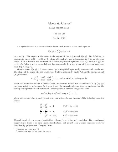
An algebraic curve is a curve which is determined by some polynomial equation
f(x,y) = ∑ a ij x i y j = 0
in x and y. The degree of the curve is the degree of the polynomial f(x,y). By definition, a
parametric curve α(t) = (p(t),q(t)), where p(t) and q(t) are polynomials in t, is an algebraic
curve. This is because the resultant of the two polynomial equations x = p(t) and y = q(t) in
terms of t (with x and y as coefficients) is a polynomial in x and y and of degree no more than
max(deg(p),deg(q)).
Given a curve f(x,y) = 0, we can often get a simplified equation by rotation and translation.
The shape of the curve will not be affected. Under a rotation by angle θ about the origin, a point
(x,y) becomes
( ) cos θ sin θ
(x,y)
= (xcos θ − y sin θ,xsin θ + y cos θ)
− sin θ cos θ
where the matrix on the left is referred to as the rotation matrix. Under a translation by (x 0 ,y 0 ),
the same point (x,y) becomes (x + x 0 ,y + y 0 ). By properly selecting θ,x 0 ,y 0 and applying the
corresponding rotation and translation, every quadratic curve in the general form
αx 2 + βxy + γy 2 + δx + ǫy + ζ = 0,
where at least one of α,β, and γ is not zero, can be transformed into one of the following canonical
forms:
x 2
a 2 + y2
b 2 = 1, if β 2 − 4αγ < 0;
x 2
a 2 − y2
b 2 = 1, if β 2 − 4αγ > 0;
y 2 = 2ax, if β 2 − 4αγ = 0.
Thus all quadratic curves are classified into ellipses, hyperbolas, and parabolas 1 . For equations of
higher degree there is no such simple classification. Let us first look at some examples of curves
described by polynomials of degree three.
∗ Materials are taken from [1].
1 These curves together are called the conics.
1

1 Some Algebraic Curves
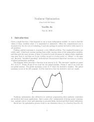
The semi-cubical parabola (i.e., a cuspidal cubic) is a cubic curve which has two branches at the
origin, but the tangents there to the two branches coincide. The origin is a cusp of the curve, and
the common limiting tangent (i.e., the x-axis) to the two branches at the cusp is called the cuspidal
tangent. See the figure below.
The algebraic equation of the semi-cubical parabola is
The parametric equation is
y 2 = x 3 .
(x,y) = (t 2 ,t 3 )
where t takes on any real value. This is a parameterization in that both x(t) and y(t) are polynomials
in t. To derive this from the algebraic equation, we consider the intersection of the curve with the
line y = tx for each fixed value of t. Substituting y = tx into y 2 − x 3 = 0 gives x 2 (t 2 − x) = 0 .
solving this gives two copies of the point (x,y) = 0, together with x = t 2 , y = tx = t 3 . Therefore
all points satisfying the algebraic equation are given by the parametric equation (x,y) = (t 2 ,t 3 ).
The polar equation is
ρ = sin 2 θ sec 3 θ, − π 2 < θ < π 2 .
This equation is obtained by substituting x = ρcos θ and y = ρsin θ into the algebraic equation.
We obtain ρ 2 (sin 2 θ − ρcos 3 θ) = 0, which gives ρ 2 = 0 and sin 2 θ − ρcos 3 θ = 0. But the second
equation subsumes the first one. From the polar equation we have
r = (ρcos θ,ρsinθ) = (tan 2 θ,tan 3 θ),
and the substitution t = tan θ yields the parametric equation.
The semi-cubical parabola is an isochronous curve; a particle descending the curve under gravity
falls equal vertical distances in an equal time (Huygens 1687). It was the first algebraic curve whose
arc length was calculated (Neile 1659). Before this the arc length had been found only for certain
transcendental curves such as the cycloid and the equi-angular spiral.
2

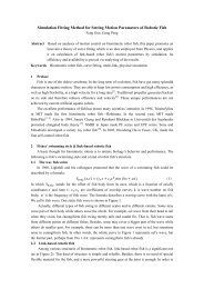
Some plane curves appear to have several parts. The simplest example of this is the hyperbola,
which has two unbounded parts that do not meet in the plane. We now give an example of a
cubic curve 2 which appears to have two parts, one of which is bounded and the other of which is
unbounded.
The algebraic equation is
A parametric equation of the curve is
y 2 − x 3 + x = 0.
x = t, y = ± √ t(t 2 − 1) −1 ≤ t ≤ 0 or t ≥ 1.
This parameterization by x is given by solving the algebraic equation to give y as a function of x.
We determine where the line x = t meets the curve for each fixed value of t. Substituting x = t
into y 2 − x 3 + x = 0 gives y 2 − t 3 + t = 0. Solving this gives x = t, y = ± √ t(t 2 − 1). This gives
parameterizations of four parts of the curves, one in each of the four quadrants. These parametric
equations are not differentiable at t = 0, ±1.
An algebraic curve can be parametrized in many different ways. An alternative parametric
equation is given by determining where the line y = tx meets the curve for each fixed value of t.
Substituting y = tx into y 2 − x 3 + x = 0 gives x(t 2 x − x 2 + 1) = 0. Solving this gives the origin
(x,y) = 0, the parameterization
r(t) = 1 (
t 2 − √ (
t
2
4 + 4,t t 2 − √ ))
t 4 + 4
of the bounded part of the curve and the parameterization
r(t) = 1 (
t 2 + √ (
t
2
4 + 4,t t 2 + √ ))
t 4 + 4
of the unbounded part. The origin is not covered by the parameterization of the bounded part,
because it corresponds to the value ∞ of the parameter, that is, to the vertical line x = 0. These
two parameterization are differentiable for all values of t.
2 The figure is taken from [1, p. 60].
3

The polar equation of the same curve is
−ρ 2 cos 3 θ + ρsin 2 θ + cos θ = 0.
This is obtained by substituting x = ρcos θ and y = ρsin θ into the algebraic equation. There are
two values of ρ corresponding to each value of θ.
2 Singular Points
A singular point of the algebraic curve f(x,y) = 0 is a point (a,b) on the curve at which
∂f
∂x = ∂f
∂y = 0,
that is at which the gradient ∇f = 0. At a non-singular point, ∇f ≠ 0. To determine singular
points, it is not sufficient to solve ∇f = 0. We must find simultaneous solutions of ∇f = 0 and
f = 0; that is, we must find those ‘singularities of the polynomial’ which also lie on the curve.
Example 1. Find the singular points of the circle f(x, y) = x 2 + y 2 − 1. From ∇f = (2x, 2y) = 0 we
obtain that x = y = 0. But (0, 0) does not lie on the circle, so the circle has no singular points.
For the cuspidal cubic g(x, y) = y 2 −x 3 = 0, we obtain that ∇g = (−3x 2 , 2y) = 0 if and only if x = y = 0.
The only singular point is (0, 0).
3 Parameterization of Algebraic Curves
Consider an algebraic curve given by f(x,y) = 0, where f is a polynomial of degree d ≥ 1. One
question is ‘Is it possible to parameterize the curve?’ We now show that algebraic curves can be
parametrized locally near non-singular points. In general, algebraic curves, or parts of them, can
be parametrized either by x or by y, or by both.
A local parameterization of an algebraic curve near a point (a,b) on the curve, is a parameterization
J → R 2 of a piece of the curve including the point (a,b). Usually we assume that the point
(a,b) corresponds to an interior point of the interval J of parameterization.
Theorem 1 (Local Parameterization Theorem) Let f be a polynomial of degree d ≥ 1 satisfying
f(a,b) = 0 and ∂f
∂y
(a,b) ≠ 0. Then there is an interval J = (a − ǫ,a + ǫ) where ǫ > 0, and
a unique smooth function φ : J → R such that φ(a) = b and f(x,φ(x)) = 0 for all x ∈ J. This
solution gives a unique regular smooth local parameterization of the curve in the neighborhood of
the point (a,b) by the x coordinate, that is, r(x) = (x,φ(x)) for all x ∈ (a − ǫ,a + ǫ). Locally, the
curve f(x,y) = 0 is the graph of the function y = φ(x), and
dφ
dx = −f x
f y
, x ∈ J.
Similarly, in the case where ∂f
∂x
(a,b) ≠ 0, there exists a unique regular smooth local parameterization
(ψ(y),y) defined near b and satisfying ψ(b) = a, f(ψ(y),y) = 0, and
dψ
dy = −f y
f x
for y near b. In the neighborhood of (a,b) the curve f(x,y) = 0 is the graph of the function
x = ψ(y).
4

The above theorem is a special case of the implicit function theorem, of which the proof can be
found in texts on analysis.
These smooth local parameterizations of algebraic curves by x or y are regular; for example,
the derivative of (x,φ(x)) is (1,φ ′ (x)) ≠ 0.
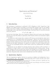
Example 2. Consider the circle given by f(x, y) = x 2 + y 2 − 1 = 0. We have f y = 2y ≠ 0 when y ≠ 0.
Thus the theorem tells us there is a local smooth parameterization by x near (a, b) where a 2 + b 2 = 1 and
b ≠ 0. Indeed the parameterization is given by
(x, √ 1 − x 2 )
or by
(x, − √ 1 − x 2 )
, −1 < x < 1
depending on whether b > 0 or b < 0. In this case, for fixed a with −1 < a < 1, there are two values for b,
and local parameterizations are given.
y
( x, 1- x 2 )
top
semi-circle
x
bottom
semi-circle
( x, - 1- x 2 )
Similarly, for a ≠ 0, there is a local parameterization by y near (a, b). Again this is given by
(√ (
1 − y2 , y)
or by − √ )
1 − y 2 , y , −1 < y < 1
depending on whether a > 0 or a < 0.
4 Curvature of Algebraic Curves
In general algebraic curves cannot be parametrized in a simple way, that is, by using a simple
formula which gives a parameterization of the whole curve. Therefore the formula for the curvature
of parametric curves cannot be used. However, according to Theorem 1 algebraic curves can be
parametrized locally near a non-singular point, though not in general using a simple formula. We
now use this result to give a parameter-free formula for the curvature of algebraic curves.
We recall that the Hessian matrix of a polynomial f(x,y) is
( )
fxx f
H = xy
.
f xy f yy
Theorem 2 The curvature of the algebraic curve f(x,y) = 0 at a non-singular point (x,y) on the
5

curve is
( )
fy
(f y , −f x )H
−f x
κ = ±
‖∇f‖ 3
= ± f2 yf xx − 2f x f y f xy + f 2 xf yy
(f 2 x + f 2 y) 3 2
= ± f2 y f xx − 2f x f y f xy + fx 2f yy
(fx 2 + ,
f2 y )3 2
where the sign ‘−’ is chosen in case the motion along the curve is in the direction of the vector
(f y , −f x ) and where the sign ‘+’ is chosen in case the motion along the curve is in the direction of
the vector (−f y ,f x ).
Proof By Theorem 1, the algebraic curve can be given a regular local parameterization near a
non-singular point by α(t) = (x(t),y(t)). Differentiating the equation
( )
f x(t),y(t) = 0,
using the chain rule, we obtain
α ′ · (f x ,f y ) = 0.
Therefore α ′ is orthogonal to (f x ,f y ), and we have α ′ = (x ′ ,y ′ ) = λ(f y , −f x ) where λ ≠ 0 is a
function of t. On differentiating once more we obtain
( )
α ′′ · (f x ,f y ) + (x ′ ,y ′ x
′
)H
y ′ = 0.
Therefore we have
x ′ y ′′ − y ′ x ′′ = α ′′ · (−y ′ ,x ′ )
Since ‖α ′ ‖ = |λ| · ‖(f y , −f x )‖, we have that
= λα ′′ · (f x ,f y )
( )
= −λ(x ′ ,y ′ x
′
)H
y ′ ( )
= −λ 3 fy
(f y , −f x )H .
−f x
κ = α′ × α ′′
‖α ′ ‖ 3 = x′ y ′′ − y ′ x ′′
‖α ′ ‖ 3
= ± f2 yf xx − 2f x f y f xy + f 2 xf yy
‖∇f‖ 3 .
Corollary 3 The algebraic curve has a point of inflection at a non-singular point (a,b) if and only
if,
f 2 y f xx − 2f x f y f xy + f 2 x f yy
is zero at (a,b) and changes sign as (x,y) moves through (a,b) along the curve.
6

Thus in order to find all points of inflection of an algebraic curve we first determine the points
where the curvature is zero by finding the simultaneous solutions of the equations
f(x,y) = 0,
f 2 y f xx − 2f x f y f xy + f 2 x f yy = 0,
and then find those solutions which are non-singular points. Next, we determine whether the
curvature changes sign as we move along the curve past the point of zero curvature. If it does, the
point is an inflection. In practice we can check on the change of sign if, for example, the curve can
be parametrized near the point by x, and
f 2 y f xx − 2f x f y f xy + f 2 x f yy
becomes a function of x after substituting from f(x,y) = 0. Such a local parameterization by x
exists by Theorem 1 provided that the tangent at the point is not parallel to the y-axis.
Example 3. Calculate the curvature of the hyperbola
at the point (2, 1).
Let f = x 2 − 3y 2 − 1. We have
Therefore
κ =
x 2 − 3y 2 = 1
f x = 2x,
f y = −6y,
f xx = 2,
f xy = 0,
f yy = −6.
± (−6y)2 · 2 + (2x) 2 · (−6)
(4x 2 + 36y 2 ) 3 2
= ± 9y2 − 3x 2
.
(x 2 + 9y 2 ) 3 2
In particular,
κ(2, 1) = ± 3
( √ 13) 3 .
Example 4. Find the points of inflection of the acnodal cubic
f(x, y) = y 2 + x 2 − x 3 = 0.
We have
f x = 2x − 3x 2 ,
f y = 2y,
f xx = 2 − 6x,
f xy = 0,
f yy = 2.
7

Eliminating y from
we have, on the curve, that
f(x, y) = y 2 + x 2 − x 3
= 0,
f 2 y f xx − 2f x f y f xy + f 2 x f yy = 4y 2 (2 − 6x) + 2(2x − 3x 2 ) 2
= 8y 2 − 24xy 2 + 8x 2 − 24x 3 + 18x 4 ,
f 2 y f xx − 2f x f y f xy + f 2 x f yy = 8x 3 − 6x 4 .
The origin is a singular point. Therefore there are precisely two points of zero curvature. They are
At these points
∇f = (2x − 3x 2 , 2y)
is not parallel to the y-axis, and therefore the curve can be parametrized locally by x. Also
8x 3 − 6x 4 = 6x 3 ( 4
3 − x )
( )
4
3 , ± 4
3 √ .
3
changes sign as we move along the curve past each of the points and therefore the curvature also changes
sign. Thus the two points are points of inflection.
References
[1] J. W. Rutter. Geometry of Curves. Chapman & Hall/CRC, 2000.
8