Simulation Fitting Method for Setting Motion Parameters of Robotic ...
Simulation Fitting Method for Setting Motion Parameters of Robotic ...
Simulation Fitting Method for Setting Motion Parameters of Robotic ...

Create successful ePaper yourself
Turn your PDF publications into a flip-book with our unique Google optimized e-Paper software.
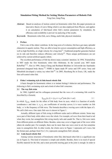
<strong>Simulation</strong> <strong>Fitting</strong> <strong>Method</strong> <strong>for</strong> <strong>Setting</strong> <strong>Motion</strong> <strong>Parameters</strong> <strong>of</strong> <strong>Robotic</strong> Fish<br />
Feng Guo, Gang Peng<br />
Abstract Based on analyses <strong>of</strong> motion control on biomimetic robot fish, this paper promotes an<br />
innovative theory <strong>of</strong> curve fitting which is an idea employed from Physics, and applies<br />
it on calculation <strong>of</strong> link-based robot fish’s motion parameters by simulation. Its<br />
efficiency and availability is proved via analyzing <strong>of</strong> the results.<br />
Keywords Biomimetic robot fish, curve fitting, multi-link, physical simulation<br />
1 Preface<br />
Fish is one <strong>of</strong> the oldest vertebrate. In the long term <strong>of</strong> evolution, fish have got many splendid<br />
characters in aquatic motion. They are able to keep low power consumption and high efficiency, as<br />
well as high flexibility, at a high velocity <strong>for</strong> a long time [1] . Traditional propeller generates backset<br />
on its side and there<strong>for</strong>e reduces efficiency and velocity [2] . These unique per<strong>for</strong>mances are not<br />
achieved by current artificial aquatic robots.<br />
The excellent per<strong>for</strong>mance <strong>of</strong> fish has drawn many scientists’ attention. In 1994, Triantafyllou<br />
in MIT made the first biomimetic robot fish—Robotuna. In the second year, MIT made<br />
RoboPike [3~4] . Also in 1994, Jianyu Cheng and Reinhard Blickhan in Universität des Saarlandes<br />
promoted elongated body theory [5] . NMRI in Japan made PF series and UPF series. Sony and<br />
Mitsubishi developed a variety toy robot fish [6] . In 2005, Huosheng Hu in Essex, UK, made the<br />
first self-control robot fish.<br />
2 Fishes’ swimming style & link-based robotic fish<br />
A basic thought <strong>for</strong> biomimetic robots is to imitate biology’s behavior and per<strong>for</strong>mance. The<br />
following is fish’s swimming style and a kind <strong>of</strong> robot fish’s structure.<br />
2.1 The way fish swim<br />
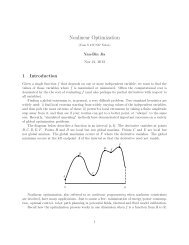
In 1960, Lighthill and his colleagues promoted that the wave <strong>of</strong> a swimming fish could be<br />
described by a <strong>for</strong>mula:<br />
, <br />
(1)<br />
In which stands <strong>for</strong> the <strong>of</strong>fset <strong>of</strong> fish body from its axes, which is a function <strong>of</strong> axially<br />
coordinates and time ; c ,c are coefficients <strong>of</strong> envelop curves; k is wave number on fish<br />
body; ω is the frequency <strong>of</strong> fish wave. The <strong>for</strong>mula describes a waving curve with the lapse <strong>of</strong> t.<br />
We call it fish wave. One static fish wave is shown in Figure 1.<br />
Actually, different types <strong>of</strong> fish swing in different scales and to different extents. Some may<br />
wave part <strong>of</strong> their body while others wave the whole. For example, eel wave from their head to tail<br />
when they swim, but carangi<strong>for</strong>m fish swing merely tails and caudal fin. That is, fish wave starts<br />
from different points on different fishes. Besides, some may cover a bigger part <strong>of</strong> the wave while<br />
others do smaller part. For example, there can be more than one wave crest in eel, but sometime<br />
none in carangi<strong>for</strong>m fish. In other words, the whole curve in Figure 1 represents eel’s wave, but<br />
the <strong>for</strong>mer part, perhaps from 0 to 1.4 , represents carangi<strong>for</strong>m fish’s already.<br />
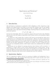
2.2 Link-based robotic fish<br />
Among various structures <strong>of</strong> biomimetic robot fish, link-based robot fish is a significant one<br />
(as in Figure 2). This kind <strong>of</strong> structure is simple and reliable. Besides, there is no need <strong>of</strong> special<br />
flexible material <strong>for</strong> the fish, and a mere powerful steering gear at the joint is enough.<br />
In order to
4<br />
3<br />
Fish wave<br />
Envelope curve<br />
2<br />
Lateral Displacement<br />
1<br />
0<br />
-1<br />
-2<br />
-3<br />
-4<br />
0 1 2 3 4 5 6 7<br />
Longitude Distance from Head<br />
Figure 1 Static fish wave<br />
Figure 2 Link-based robot fish<br />
make the machine swim like a fish, we should set parameters, such as angle at the joint, proportion<br />
<strong>of</strong> each rod, one segment <strong>of</strong> link, so that the link mimics fish’s shape as well as possible.<br />
3. Traditional strategy in fitting fishcurve with link<br />
Traditional method is widely used. It is simple, but there are also some flaws in it.<br />
3.1 Preparation <strong>for</strong> fitting fish curve<br />
Suppose the robot fish acts N times in a period with equal interval. Then, a period should be<br />
discretized into N time points. So at each point, fish wave degenerate into N static curves. We may<br />
call them fish curves.<br />
For 2/;i=0,1...N-1; <strong>for</strong>mula <strong>of</strong> fish curve i should be:
’ , <br />
(2)<br />
<br />
When N=12, the 12 curves are shown in Figure 3.<br />
<br />
2<br />
1.5<br />
1<br />
Lateral Displacement<br />
0.5<br />
0<br />
-0.5<br />
-1<br />
-1.5<br />
-2<br />
0 0.5 1 1.5 2 2.5 3 3.5 4 4.5<br />
Longitude Distance from Head<br />
Figure 3 Fish curves on 12 time points<br />
After time discretization, we can fit the curves one by one. The fishcurve with 0 phase, that is<br />
the first fishcurve, is picked <strong>for</strong> the following work.<br />
3.2 Joint Location <strong>Method</strong><br />
Just as stated be<strong>for</strong>e, because <strong>of</strong> different swing styles, we must know which part <strong>of</strong> a fish<br />
curve is to be fitted by robot fish. Suppose the part is from 0 to 2π*R(R>0). The size <strong>of</strong> R affects<br />
fish pushing ability and speed significantly. In this article, set R=0.7 according to our robot fish.<br />
Current fitting strategy that is commonly seen is to locate every joint on the fish curve, and<br />
ensure the link’s length matches the curve. Then we get the result. We may call this method “Joint<br />
Location <strong>Method</strong>” (JLM).<br />
JLM is simple and reliable, but there are some flaws in it. When the derivative <strong>of</strong> a fish curve<br />
remains the same sign, that is, when it’s convex or concave, this method will cause certain<br />
accumulative error, and the link we get will distribute on one side <strong>of</strong> the curve. As a result, the gap<br />
between link and curve is relatively large. As in Figure 4, the blue dashed line represents a fish<br />
curve with 0 phase, and the red line represents the link we get with this method. We can see that<br />
almost the whole link locates beneath the fish curve. So it is the situation with other phases. This<br />
result not only distorts the shape <strong>of</strong> the curve, but also decreases its amplitude. And there<strong>for</strong>e may<br />
affect robot fish’s swimming quality.<br />
3.3 Other way <strong>of</strong> fitting<br />
An easily thought <strong>of</strong> way to fix the problem is to integrate the difference between fish wave
0.5<br />
Fish curve<br />
Link<br />
0<br />
Lateral Displacement<br />
-0.5<br />
-1<br />
-1.5<br />
-2<br />
0 0.5 1 1.5 2 2.5 3 3.5 4 4.5<br />
Longitude Distance from Head<br />
Figure 4 Result by JLM<br />
and link and make the outcome minimum. However, there are even more problems in this method.<br />
First <strong>of</strong> all, there is no obvious guide <strong>for</strong> adjustment in intermediate states. So there is only one<br />
way to find the result, searching thoroughly. Then it causes another problem: high computational<br />
complexity, especially when there are many segments in the link. So we need to figure out another<br />
method.<br />
4 <strong>Simulation</strong> <strong>Fitting</strong> <strong>Method</strong><br />
It is necessary to find a method which can compromise between computational complexity<br />
and precision. Just as we borrow the structure <strong>of</strong> real fish to design robot fish, we can also borrow<br />
ideas from physics to reach our goal.<br />
4.1 Principle <strong>of</strong> the method<br />
The basic thought <strong>of</strong> SFM is simple: view the fishcurve and link as real objects, imagine a<br />
uni<strong>for</strong>m <strong>for</strong>ce field between them and let physic laws do the rest.<br />
As in Figure 5, a series <strong>of</strong> elastic ropes (shown as black lines) are attached between the link<br />
and fish curve. Suppose the ropes always satisfy Hook Law and tend to contract. Then, in an<br />
unstable state, rods are subjected to certain <strong>for</strong>ce and torque which drive them to translate and<br />
rotate. Under such effect, link moves to its target position and finally stops in a stable state. Now,<br />
the shape <strong>of</strong> the link is right <strong>for</strong> robot fish. All we need to do is to build a mathematic model,<br />
simulate the process and record the result.<br />
4.2 Physical modeling and analysis<br />
With the set scene, it is easy to analyze the system.<br />
4.2.1 Analyze single rod
0.5<br />
0<br />
Lateral Displacement<br />
-0.5<br />
-1<br />
-1.5<br />
Fish curve<br />
Link<br />
-2<br />
0 0.5 1 1.5 2 2.5 3 3.5 4 4.5<br />
Longitudinal Distance from Head<br />
Figure 5 <strong>Simulation</strong> <strong>Fitting</strong> <strong>Method</strong><br />
According to their moving pattern, the rods should be divided into 2 categories: (1) head static<br />
but tail free, that is, the first rod; (2) both head and tail free, that is, all rods except the first.<br />
Analyze the 2 categories separately. Suppose a rod with dip α is subjected to erect <strong>for</strong>ce with<br />
distribution density at x (as in Figure 6). The acceleration <strong>of</strong> the head is a and its angular<br />
acceleration is .<br />
Figure 6 Force analyses on rod<br />
(1) For head static, but tail free rod.<br />
Because <strong>of</strong> its static head, rod can just rotate. Then a=0. Let’s take a look into β. According to<br />
law <strong>of</strong> rigid-body rotation:<br />
<br />
<br />
(3)
In which, , each represents the head and tail <strong>of</strong> the rod; J represents moment inertia, and in<br />
this situation where rigid even rod rotate surrounding its end, 。<br />
Then:<br />
(2) For both head and tail free rods.<br />
According to Newton second law:<br />
And work energy relationship:<br />
<br />
<br />
<br />
<br />
<br />
<br />
<br />
(4)<br />
<br />
<br />
<br />
<br />
<br />
<br />
(5)<br />
<br />
Then we get:<br />
<br />
<br />
<br />
<br />
<br />
<br />
<br />
(6)<br />
<br />
<br />
<br />
<br />
<br />
<br />
<br />
<br />
<br />
<br />
<br />
<br />
<br />
<br />
<br />
<br />
<br />
<br />
<br />
<br />
<br />
<br />
<br />
<br />
(7)<br />
<br />
<br />
(8)<br />
<br />
If we simulate w ith equal step, in one step, rod’s shift is proportional to and its rotate angle to .<br />
4.2.2 Analyze the link<br />
An obvious fact is that the link must not be broken, so the tail <strong>of</strong> a <strong>for</strong>mer rod should keep<br />
pace with the head <strong>of</strong> the latter one. In this way, the plain shift <strong>of</strong> the latter<br />
one will cause rotation<br />
on the <strong>for</strong>mer one. Since the shift in every step is much smaller than the rod’s length, the rotation<br />
angle is proportional to <strong>of</strong> the latter one. Suppose ∆ is the modifying rotation angle caused<br />
by this effect, then:<br />
∆ ∆ / <br />
(9)<br />
In which ∆ represents the plain shift <strong>of</strong> the latter rod; represents the length <strong>of</strong> the <strong>for</strong>mer. So<br />
far we have calculated all crucial parameters <strong>of</strong> the model.<br />
4.3 Experimental modeling and simulation<br />
According to the physical model above, it’s easy to program and simulate with equal step<br />
method in Matlab. When the precision comes to certain range, result is got. Flowchart <strong>of</strong><br />
simulation program is shown as Figure 7. The result <strong>of</strong> simulation is shown as Figure 8.<br />
With SFM, we can repeat the simulation and get link shape at other time points one by one<br />
and finally get every shape.<br />
5 Comparison and Analysis<br />
JLM per<strong>for</strong>ms well when the second derivative <strong>of</strong> the curve varies slightly, that is when curve<br />
is close to straight line. Nevertheless, in general, accumulated error is unavoidable, especially<br />
when the curve is concave or convex function.<br />
SFM avoids that kind <strong>of</strong> error theoretically, and gets similar amplitude with the original curve.<br />
Of course, different factors always violate each other. When the curve is close to straight line, the<br />
link we get doesn’t stick tightly to the curve; instead, there is a small gap, which, in fact, can be<br />
neglected. Besides, the computational complexity <strong>of</strong> SFM is a little higher than that <strong>of</strong> JLM.<br />
Table 1 gives 2 kinds <strong>of</strong> error by the two methods. Linear error (err) is the integral <strong>of</strong>
Figure 7 <strong>Simulation</strong> flow chart<br />
0.5<br />
Fish curve<br />
Link<br />
0<br />
teral Displacement<br />
La<br />
-0.5<br />
-1<br />
-1.5<br />
-2<br />
0 0.5 1 1.5 2 2.5 3 3.5 4 4.5<br />
Longitude Distance from Head<br />
Figure 8 Result by SFM<br />
difference between link and fish curve, calculated with the following <strong>for</strong>mula:<br />
<br />
(9)<br />
<br />
In which represents the shift <strong>of</strong> fish curve, and is the shift <strong>of</strong> link. Square error (serr) is the<br />
integral <strong>of</strong> the second power <strong>of</strong> the difference, calculated with the following <strong>for</strong>mula:<br />
<br />
<br />
<br />
<br />
<br />
<br />
(10)
Table 1 Error comparison<br />
Linear error<br />
Square error<br />
JLM SFM JLM SFM<br />
1 282.7539 -31.6493 117.5796 74.4139<br />
2 299.8585 -18.6237 135.8531 86.8413<br />
3 244.7837 -10.0649 116.8211 75.6017<br />
4 169.971 11.6239 71.1852 42.3516<br />
5 59.8206 40.3002 33.7386 18.1548<br />
6 45.0723 0.574 39.2045 20.1163<br />
7 8.744 -4.4178 34.7495 15.3578<br />
8 -63.6139 21.0387 22.7306 8.5813<br />
9 -101.151 50.1628 24.9156 11.4755<br />
10 -150.719 56.1411 36.8875 19.145<br />
11 -176.029 53.2019 53.8563 32.5745<br />
12 -241.814 42.7809 85.025 52.4728<br />
13 -282.754 30.299 117.5796 74.5112<br />
14 -299.859 18.684 135.8531 86.8327<br />
15 -244.784 10.0424 116.8211 75.6027<br />
16 -167.971 -11.6179 71.1852 42.3517<br />
17 -59.8206 -40.2987 33.7386 18.1547<br />
18 -45.0723 -0.5738 39.2045 20.1164<br />
19 -8.744 4.4176 34.7495 15.3578<br />
20 63.6139 -21.04 22.7306 8.5813<br />
21 101.1514 -50.1645 24.9156 11.4757<br />
22 150.7191 -56.146 36.8875 19.1454<br />
23 176.029 -53.1993 53.8563 32.5744<br />
24 241.8141 -42.7759 85.025 52.4725<br />
From table 1, we can see, on 24 discrete time points, the errors with simulation fitting method<br />
are all smaller than those with JLM. The linear error <strong>of</strong> the <strong>for</strong>m er ranges 1.27%~67.37% <strong>of</strong> the<br />
latter, with an average <strong>of</strong> 26.26%; the rate with square error i s 7.75% ~64.71% , with an average <strong>of</strong><br />
54.89%。<br />
6 Conclusion<br />
This article promotes an innovativ e method, simulation fitting method, in orde r to reduce<br />
the difference betwee n link and fish curve. Two points feature this me thod : first, it is borrowed<br />
from physics phenomenon, so we need n’t to worry about its astringency an d stability; second, <br />
and give out adjusting direction in simulation, and there<strong>for</strong>e avoid unacceptable calculation<br />
amount. Mo reover, this method can also be used whenever l ink is used to tak e the <strong>for</strong>m <strong>of</strong> curve.<br />
Nevertheless, we didn’t test its per<strong>for</strong>mance with fluid mechanics, but most likely, the result
will show its excellence only i n high speed swimming. I n further study, a test on swimming<br />
per<strong>for</strong>mance <strong>of</strong> the re sult should be made, including both simulation a nd real robot fish test.<br />
Reference<br />
1 Zhang Yiming, Zhan Xingqun, Zhang Yanhu a. Research on motion rules <strong>of</strong> biomimetic robot f ish. China Ship<br />
Building, 2006,47:174.<br />
2 Zhang Yi, Yang Ruimin, W angzhou, Liu Huan, Zhou Guang . Overview <strong>of</strong> research on robot fish. Journal <strong>of</strong><br />
Chongqing Post and Telegraph University (Scien ce version) , 2007, 19:5.<br />
3 MS Triantafyllou, DS Barr ett, DKP Yue, JM Anderson, MA Grosenbaugh, K. Streitlien, and GS Triantafyllou. A<br />
new paradigm <strong>of</strong> propulsion and maneuvering <strong>for</strong> marine vehicles. SNAME T rans, 1996 (104): 81-100.<br />
4 MS Triantafyllou, S Michael, & S George. An efficient swimming<br />
machine. Scientific American,<br />
1995,272(3):64-70.<br />
5 J Y Cheng, R Blickhan. Note on the calculatio n <strong>of</strong> propeller Efficiency using elongated body theory. J Exp Biol,<br />
1994 (192): 169-177.<br />
6 Yu Junzhi, Chen Erqui, Wang Shuo, T an Min. Analyses and progress <strong>of</strong> biomemetic robot fish. Control theory<br />
and application, 2003,20:4.