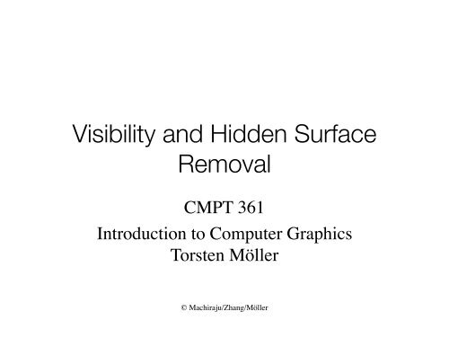
Visibility and Hidden Surface Removal

Visibility and Hidden Surface 

Removal 

CMPT 361 

Introduction to Computer Graphics 

Torsten Möller 

© Machiraju/Zhang/Möller

Rendering Pipeline 

Hardware 

Modelling Transform Visibility 

Illumination + 

Shading 

Perception, 

Interaction 

© Machiraju/Zhang/Möller 

Color 

Texture/ 

Realism

Reading 

• Angel – Chapter 6.10-6.11, 8.11 

• Foley et al – Chapter 15 

• Shirley+Marschner – Chapter 12 


3

Visibility 

• Polygonal model - a collection of vertices 


4

Visibility (2) 

• Connecting dots (wireframe) helps, 

• but it is still ambiguous 


5


• Visibility helps to resolve this ambiguity 


6


• Include shading for a better sense of 3D 


7


• Another Example 


8


• wireframe 


9


• Inner object visibility 

Back-Face Culling 


10


• Inter-object visibility 


11


• Shading 


12

Why compute visibility? 

• Realism: Occlusions make scenes look more 

realistic 

• Less ambiguity: Visibility computations 

provide us with depth perception 

• Efficiency: Rendering is time consuming, so 

we should not have to waste time on objects 

we cannot see © Machiraju/Zhang/Möller 

13

Visibility + shading 

• Visibility is only one aspect for realistic 

rendering 

• Visibility + shading → even better sense of 

3D 


14

Classification of algorithms 

• Hidden surface removal (HSR) vs. visible surface 

determination (VSD) 

– HSR: figure out what cannot be seen 

– VSD: figure out what can be seen 

• Image space vs. object space algorithms 

– Image space: per pixel based (image precision) ― 

determine color of pixel based on what is visible, 

e.g., ray tracing, z-buffering 

– Object space: per polygon or object based in object 

space (object precision), eg, back to front (depth sort) 

– In many cases a hybrid of the two is used 


15

Image Space 

For each pixel in image { 

determine the object closest to the 

viewer, pierced by the projector 

through the pixel 

draw the pixel using the appropriate 

colour 

} 

• dependent on image resolution 

• simpler, possibly cheaper 

• aliasing a factor 


Object Space 

for each object in world { 

determine those parts of objects 

whose view is unobstructed by 

other parts of it or other objects 

draw those parts in the appropriate 

colour 

} 

• independent of image resolution 

• More complex 3D interactions 

• Can be more expensive, e.g., subdivision 

• designed first for vector displays 


Visibility is expensive 

• Image space – brute-force 

– O( #pixels * #objects) 

– 1286 x 1024 resolution and 1 million polygons 

– Complexity: O(1.3 x 10 12 ) 

• Object space – brute-force 

– Worst-case: each object compared with the 

others 

– Complexity: O(n 2 ), e.g., 1 million polygons → 

O(10 12 ) 


18

How to improve efficiency 

• Pay attention to order in which primitives 

are processed, e.g., if back to front then just 

“paint” 

• Be as lazy as possible! 

– Costly operations are to be avoided as much as 

possible, e.g., use of bounding boxes 

– Try to make use of previous computations, e.g., 

utilize coherence 

• Specifically … 


19

Efficient visibility techniques 

• Coherence 

• Use of projection normalization 

• Bounding boxes or extents 

• Back-face culling 

• Spatial partitioning or spatial subdivision 

• Hierarchy 


20

1. Coherence 

• Why? — Object properties, e.g., 

– geometry, color, shading, and 

– visibility situations 

often vary smoothly – local similarities 

• Utilizing coherence: reuse computations 

made for one part of an object for nearby 

parts 

– without change or 

– with only incremental updates 


21

1. Object and area coherence 

• Object coherence 

– if two objects are well separated, 

only one comparison is needed 

between objects and not between 

their component faces 

• Area coherence: 

– group of adjacent pixels likely 

covered by the same visible face 


22

1. Edge and face coherence 

• Edge coherence 

– an edge changes visibility only where it crosses a visible 

edge or when it penetrates a visible face 

• Implied edge: 

– line of intersection of two planar faces can be determined 

from two intersection points 

• Scan-line coherence 

– visibility information will likely change little between 

adjacent scan lines 

• Face coherence 

– Surface properties will likely vary smoothly across a face, 

so calculations on © a Machiraju/Zhang/Möller 

face may be modified incrementally 

23

1. Depth and frame coherence 

• Depth coherence 

– once the depth of one surface point is 

computed, the depth of the rest of the surface 

can be found from a difference equation (e.g., 

in z-buffer) – adjacent parts of a face have 

similar depth values 

• Frame coherence 

– images in a sequence (e.g., animation) will 

likely change little from one to the other, so can 

reuse information from current frame – key to 


compression 24

2. Use of projection 

normalization 

• Want to determine whether point P 1 

obscures P2 

• Need to see whether two points are on the 

same projector 

• With our projection 

normalization, just 

need to check the x 

and y’s of P’ 1 and P’ 2 


25

2. Perspective Transform 

• Parallel projection - just check (x,y) values 

(need canonical volume!) 

• perspective - more work! 

• need to check if 

x 1 /z 1 = x 2 /z 2 and 

y 1 /z 1 = y 2 /z 2 . 


26

2. Perspective Transform 

• Can bring canonical view-volume into 

screen coordinates 


3. Bounding Objects 

• Operations with objects are expensive! 

• Can we do a quick test with an 

approximation of the object? 

• Answer - yes! 

• Technique - approximation through 

“bounding volumes” or “extents” 

• avoid unnecessary clipping 

avoid unnecessary comparisons between 

objects or their projections 


28

3. Bounding Objects (2) 

• For rendering of projected polygons. If 

extents do not overlap, neither should the 

polygons 


29


• If the extents overlap then either one of the 

following cases will apply 

• Typically further subdivision 


30


• rectangular extents => bounding boxes, or 

bounding volumes in 3D 

– in general there are many possible bounding 

boxes 

– want to choose one that is efficient for a 

particular application (i.e. axis-aligned) 

– Besides comparing between objects, also used 

in ray-object intersection tests 

• spherical extend => bounding sphere 


31


• can be used in a single dimension 

• no overlap between two objects if zmax2 < 

z min1 or z max1 < z min2 

• minmax testing 

• difficult part: 

find z-extensions 


32

4. Back-face culling 

• Assumption: Objects are solid polyhedra, 

i.e., opaque faces completely enclose its 

volume 

• If viewed from outside, only exterior is 

visible 

• So we see only faces 

whose surface normals 

point towards us 


33

4. Back-face culling 

• Simple test (when looking down the −z 

axis): examine the sign of the z component 

of the surface normal 

• z < 0 in VCS → back-facing polygon 

• How effective is it? 

– Can cull about 50% polygons 

in a typical scene 

– Does not really do occlusion 

– Many invisible faces still 

processed © Machiraju/Zhang/Möller 

34

5. Spatial Partitioning 

• break a larger problem down into smaller 

ones, by assigning objects to spatially 

coherent groups as a preprocessing step 

– 2D - use a grid on the image plane 

– 3D - use a grid over object space 

– Adaptive partitioning techniques for irregularly 

distributed objects in space: size of partitions 

vary 

• Quadtrees, octrees 

• BSP-trees (binary space partition trees) 


• kd-trees 

35

5. Spatial Partitioning (2) 


36

6. Hierarchy 

• Use (e.g., semantic) information in the 

modeling hierarchy to restrict the need for 

intersection tests at lower levels, when 

children are part of parent in hierarchy, e.g., 

• Bounding boxes, spatial partitioning, 


hierarchy all use very similar ideas 

37

Visibility algorithms 

• Image-space algorithms using coherence 

– z-buffer algorithm – use of depth coherence 

– Scanline algorithm – use of scanline and depth 

coherence 

– Warnock’s (area subdivision) algorithm – use of 

area coherence and spatial subdivision 

• Object-space algorithms 

– Depth sort – use of bounding or extent 

– Binary space partitioning (BSP) algorithm 


38

z-buffer algorithm revisited 

• One of the simplest and most widely used 

• Hardware & OpenGL implementation 

common 

glutInitDisplay(GLUT_RGB | GLUT_DEPTH); 

glEnable(GL_DEPTH_TEST); 

• Use a depth buffer to store depth of closest 

object encountered at each position (x, y) on 

the screen – depth buffer part of the frame 

buffer 

• Works in image © space Machiraju/Zhang/Möller and at image precision 

39

The z-buffer algorithm 

initialize all pixels to background colour, depth to 0 

(representing depth of back clipping plane) 

for each polygon { 

for each pixel in polygon's projection { 

pz = depth of projected point 

if (pz >= stored depth) { 

store new depth pz 

draw pixel 

} 

} 

} 


40

z-buffer: exploiting depth 

coherence 

• Polygons are scan-converted as before, but 

now need to compute depth values z 

• Assume planar polygons. On scanline y, 

increment x: 

Ax + By + Cz + D =0 

z = 

z x = 

z x =z 

Ax + By + D 

C 

A(x + x + By + D 

A 

C 

x 

C 


Typically, Δx = 1 

41

z-buffer: exploiting depth 

coherence 

• From one scanline (y) to the next (y + 1): 

left polygon edge point: from (x, y) to (x + 1/m, y+1), 

where m is the slope of the polygon edge 

• So the new z 

A 

z x =z 

C 

z y =z 

A/m + B 

C 


Pre-computed 

and stored 

42

z-buffer: bilinear interpolation 

• If the polygon is non-planar, or not analytically 

defined, it is possible to approximate using bilinear 

interpolation 

Depth values 

known at vertices 

Interpolate 

between them then 

on scanline 

• Not just for depth, can do it for color (Gouraud 

shading), surface normals, or texture coordinates 

• Subdivision or refinement may be necessary is error 

is too great 


43

Depth sort algorithm 

• Determine a visibility (depth) ordering of objects 

which will ensure a correct picture if objects are 

rendered in that order – object-space algorithm 

• If no objects overlap in depth z, it is only 

necessary to sort them by decreasing z (furthest to 

closest) and render them – back-to-front rendering 

with painters algorithm 

• Otherwise, it may be necessary to modify objects, 

e.g., by intersecting and splitting polygons, to get 

depth order 


List Priority (2) 

• Depth comparisons and object splitting are 

done with object precision and the scan 

conversion is done with image precision 

• Depth Sort 

– Sort all polygons according to their smallest 

(furthest) z 

– Resolve any ambiguities (by splitting polygons 

as necessary) 

– scan convert each polygon in ascending order 

of smallest z (back to front) 


45


• Painter’s algorithm 

– simple depth sort 

– considers objects on planes of constant z (or 

non-overlapping z) 

– does not resolve ambiguities 

• Consider the following cases where 

ambiguities exist: 


46


• Do extents in z overlap? 


47


• Do polygons penetrate one another? 


48


• Do polygons cyclically overlap? 


49


• Five tests for visibility: 

– 1. do x-extents not overlap? 

– 2. do y-extents not overlap? 

– 3. is P entirely on the opposite side of Q's plane, 

from the viewpoint? 

– 4. is Q entirely on the same side of P's plane, 


– 5. do the projections of polygons onto the xy 

plane not overlap? 


50


• If these tests fail, P obscures Q. However, 

we can test if Q obscures P (so that the 

order in the list can be switched to scanconvert 

Q first) in the following way 

(replacing steps 3 and 4): 

– is Q entirely on the opposite side of P's plane, 


– is P entirely on the same side of Q's plane, from 

the viewpoint? 


51


• More examples - 

– Test 3 is true for the following 


52


• More examples - 

– Test 3 is false, test 4 is true for the following 


53

Scanline algorithm 

• Operate at image precision 

• Unlike z-buffer, which works per polygon, this 

one works per scanline 

• Avoid unnecessary depth calculations in z- 

buffer 

– Depth compared only when new edge is 

encountered 

• An extension of the polygon scan-conversion: 

deal with sets of polygons instead of just one 

• Less memory-intensive than z-buffer, but more 


complex algorithm 54

Scanline: data structure 

• Recall the polygon scan-conversion 

algorithm 

– Edge table (ET): stores non-horizontal and 

possibly shortened edges at each scanline with 

respect to lower vertex 

– Active edge table (AET): A linked list of active 

edges with respect to the current scanline y, 

sorted in increasing x 

• Extra: Polygon table (PT): stores polygon 

information and referenced from ET 


55

Scanline: data structure 

x_lower 

y_upper 


56

Scanline Example 

• Another representation of our two polygons, 

intersected with the plane associated with a 

scanline 


57

Scanline: scan example 1 

• At scanline y = a: AET has AB and AC 

– Render background color 

– At AB: invert in-out flag of ABC 


Scanline coherence – 

no depth updates yet 

– Render “in” polygon ABC using information 

from PT 

– At AC: invert in-out 

flag of ABC 

– Render background 

color 

– Next scanline 

58


• At scanline y = b: AET has AB, AC, FD, FE 

– Render background color 

– At AB: invert in-out flag of ABC 

– Render “in” polygon ABC using information 

from PT 

– At AC: invert in-out 

flag of ABC 

– Render background 

– Repeat for FD & FE 

– Next scanline 


59


• At scanline y = g: AET has AB, DE, BC, FE 

– Render background color and then ABC as 

before 

Computed 

incrementally 

as in z-buffer 

– At DE: invert in-out flag of DEF; check depth 

information of “in” polygons (ABC and DEF in a 

list of “in” polygons) 

– Render DEF 

– At BC: still render DEF 

if no penetration 

– At FE: go background 

– Next scanline © Machiraju/Zhang/Möller 

60


• Maintain a list of “in” polygons 

• Check depth information when entering into 

a new “in” polygon 

• If no penetration, 

there is no need to 

check depth when 

leaving obscured 

(occluded) polygons 


61

Scanline: polygon penetration 

• If the polygons penetrate, additional processing 

is required: e.g., introduce a false edge L’M’ 

• Such “self-intersections” should be avoided in 

modeling and detected beforehand – meshes 

are mostly OK © Machiraju/Zhang/Möller 

62

Scanline problems 

• Beware of large distances and large 

polygons with the z-buffer algorithm. 

• Problems with perspective projection can 

arise 

• the visible 

polygon 

may not 

be correctly 

determined 


63

BSP algorithm 

• Binary space partitioning of object space to 

create a binary tree – object-space algorithm 

• Tree traversal gives back-to-front ordering 

depending on view point 

• Creating/updating the tree is time- and 

space-intensive (do it in preprocessing), but 

traversal is not – efficient for static group of 

polygons and dynamic view 

• Basic idea: render polygons in the half- 


space at the back first, then front 64

Building the BSP trees 

• Object space is split by 

a root polygon (A) and 

with respect to its 

surface normal (in front 

of or behind the root) 

• Polygons (C) which lie 

in both spaces are split 

• Front and back 

subspaces are divided 

recursively to form a 


binary tree 65 

B 

D 

C 1 

C 2 

A 

E 

B E 

front back back 

C 1 

front 

A 

back 

D C 2

BSP trees traversal 

DrawTree(BSPtree, eye) { 

if (eye is in front of root) { 

DrawTree(BSPtree→back, eye) 

DrawPoly(BSPtree→root) 

DrawTree(BSPtree→front, 

eye) } 

else { 

DrawTree(BSPtree→front, eye) 

DrawPoly(BSPtree→root) 

DrawTree(BSPtree→back, eye) } 

} 


66

BSP traversal example 

• Rendering order: 

• D, B, C1, A, E, C2 

• E, C2, A, D, B, C1 

C 2 

B 

A 

C 1 

D 

View point 

E 

A 

front back 

B E 

front back back 

C 1 

D C 2 


Area subdivision 

• Divide-and-conquer and spatial partitioning 

in the projection plane. Idea: 

– Projection plane is subdivided into areas 

– If for an area it is easy to determine visibility, 

display polygons in the area 

– Otherwise subdivide further and apply decision 

logic recursively 

– Area coherence exploited: sufficiently small 

area will be contained in at most a single visible 

polygon 


68

Warnock’s subdivision 

• Divide the (square) screen into 4 equal 

squares. 

• There are 4 possible relationships between 

the projection of a polygon and an area 


69

Warnocks Algorithm (2) 

– All Disjoint: background colour can be 

displayed 

– One intersecting or contained polygon: fill with 

background and then scan-convert polygon 

inside area 


70

Warnocks Algorithm (3) 

– Single surrounding polygon: fill with colour 

from surrounding polygon 

– More than one polygon intersecting, contained 

in, or surrounding, but 1 surrounding polygon 

in front of others: fill with colour from front 

surrounding polygon (see below) 


71

Warnock’s Algorithm 

• How to determine that case 4 applies (no 

polygon penetration)? 

– Check for depth values of all planes of the polygons 

involved at the four corners of the square area 

– If a surrounding polygon wins at all four depth 

values 


72

Warnock’s Algorithm 

• If none of the cases 1 – 4 apply, the area is 

subdivided 

• If none of the cases 1 – 4 is true and cannot 

subdivide any more, e.g., at pixel precision, 

(that is unlucky) then we can assign a color 

of the closest polygon from the center of the 

pixel for example 


73

Warnock’s: example 


74

Final issues on area subdivision 

• Warnock’s algorithm subdivide using 

rectangles 

• It is possible to divide by polygon boundaries 

– Weiler-Atherton algorithm ([F] Section 

15.7.2) 

• Can even do area subdivision at subpixel level 

– Expensive obviously – full area-subdivision 

visibility at each pixel 

– Why? Use average color from all polygons that 

cover a pixel – antialiasing technique (later in the 


course) 

75

Visibility and Hidden Surface Removal

You also want an ePaper? Increase the reach of your titles

Delete template?

Save as template?