Interpretation Report for the Geotech VTEM and ... - Geology Ontario

Interpretation Report
for the
Geotech
VTEM and Magnetic
Helicopter Geophysical Surveys
of the
Broke Back and Riverbank Blocks
McFauld’s Lake Area
Ontario, Canada
on behalf of
Melkior Resources Inc.
SCOTT HOGG & ASSOCIATES LTD August 2010

TABLE OF CONTENTS
1 INTRODUCTION ............................................................................................2
2 SURVEY AREA ..............................................................................................2
3 AIRBORNE SURVEY DATA ..........................................................................3
3.1 Magnetometer .........................................................................................3
3.2 VTEM Electromagnetic System .............................................................3
3.3 B-Field and dB/dt Profiles ......................................................................6
3.4 VTEM System Geometry and Response Shape ...................................7
4 COMPILATION and PRESENTATION ..........................................................9
4.1 Time Constant Tau Calculation .............................................................9
4.2 Conductance Calculation.......................................................................9
4.3 Pole Reduced Vertical Magnetic Gradient ............................................9
4.4 Apparent Magnetic Susceptibility Map ...............................................10
5 INTERPRETATION OVERVIEW ..................................................................11
6 DISCUSSION AND RECOMMENDATIONS.................................................13
6.1 Broke Back Block .................................................................................13
6.2 Riverbank Block....................................................................................13
7 APPENDIX I : Maps and Figures ................................................................15
1

1 INTRODUCTION
Melkior Resources Inc. carried out a helicopter electromagnetic and magnetic survey
over their properties near McFauld’s Lake area of Ontario. The survey was flown by
Geotech, using the VTEM transient electromagnetic system, in May, 2010. The
geophysical survey data was provided to Scott Hogg & Associates Ltd. for analysis and
interpretation.. The interpretation process and ensuing recommendations are included in
this report.
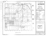
2 SURVEY AREA
The survey consists of two survey blocks, designated Broke Back and Riverbank. The
map below 1 illustrates the survey location.
2

3 AIRBORNE SURVEY DATA
The survey was carried out by Geotech. The helicopter towed geophysical system
included electromagnetic and magnetic instrumentation as follows:
3.1 Magnetometer
An optically pumped cesium sensor recorded the total magnetic field. The sensor was
towed 13 metres below the helicopter at a nominal terrain clearance of 61 metres.
Diurnal corrections were carried out by Geotech. Grids of total magnetic field were
provided.
3.2 VTEM Electromagnetic System
The VTEM system uses a superimposed dipole configuration with the receiver located
within the transmitter loop. The transmitter axis is vertical (Z). The receiver has a single
vertical axis. The transmitter current waveform is a triangular ramp, repeated with
reversing polarity, a base frequency of 30 Hz. The receiver measures the secondary
field at intervals after the termination of the transmitter current pulse. The system was
towed 45 metres below the helicopter at a nominal terrain clearance of 30 metres.
Transmitter Radius: 25.5 m.
Number of Turns: 4
Peak Current: 172 A
Tx Dipole Moment 365,279 Amps*m 2 (nIA)
Z Receiver Radius 1.2 m.
Number of Turns 100
3

Figure 1: VTEM System: The
derivative of the transmitted
waveform, or dBp/dt, is illustrated as
red line. This positive pulse is
followed by one with reverse polarity,
for a repetition rate of 30 Hz.
The location of the Off-time
measurement channels is shown in
blue.
The irregular, toothed nature of the
waveform represents an actual
measurement by the receiver.
The units of measurement for electromagnetic systems must be scaled to the primary
field. The method adopted by Geotech for the VTEM system conveniently provides for
changes in hardware for both the transmitter and receiver. The strength of the primary
field, as generated by the transmitter, is accommodated by transmitted dipole moment
which is the product of the number of coil turns, the current and the coil area.
Tx Dipole Moment = 365,279 Amps*m 2 (nIA)
The effectiveness or natural gain of the receiver is a function of its area and number of
turns.
Receiver gain
= 113.04 m 2 (nA)
The scaling factor for the system is the product of these two terms
System Scale Factor = 41,276,527 Amps*m 4 (nIA 2 )
The units of the secondary field recorded by the system are defined relative to this
system scale factor in units of picoVolts / Ampers*m 4 . By this means the VTEM units of
measurement are made independent of transmitter current as well as the size and
number of turns of both the transmitter and receiver antennae.
4

VTEM Decal Sampling Scheme (microseconds)
Index (Channel) Middle Start End Window Width
14 96 90 103 13
15 110 103 118 15
16 126 118 136 18
17 145 136 156 20
18 167 156 179 23
19 192 179 206 27
20 220 206 236 30
21 253 236 271 35
22 290 271 312 40
23 333 312 358 46
24 383 358 411 53
25 440 411 472 61
26 505 472 543 70
27 580 543 623 81
28 667 623 716 93
29 766 716 823 107
30 880 823 945 122
31 1010 945 1086 141
32 1161 1086 1247 161
33 1333 1247 1432 185
34 1531 1432 1646 214
35 1760 1646 1891 245
36 2021 1891 2172 281
37 2323 2172 2495 323
38 2667 2495 2865 370
39 3063 2865 3292 427
40 3521 3292 3781 490
41 4042 3781 4341 560
42 4641 4341 4987 646
43 5333 4987 5729 742
44 6125 5729 6581 852
45 7036 6581 7560 979
5

3.3 B-Field and dB/dt Profiles
A primary electromagnetic field is created by the current flowing in the transmitter loop.
It induces current flow in the underlying ground, which in turn, creates a secondary
electromagnetic field. This secondary magnetic field "B" induces a voltage in the reciever
which is proportional to dB/dt, the rate of change of the secondary field passing through
the coil. Geotech does not elaborate but the B field is derived by either digtal or
electronic integration of the directly measured signal dB/dt.
The basis time-domain electromagnetic anomaly can be expressed as an exponential.
B = ke -t/τ
where B is the amplitude of the B-field signal, k is a constant related to the size, shape
and depth of the source, t is time in microseconds and τ is the time-constant Tau. A
large conductive body will have a large Tau and thus the signal will decay slowly. A
small poor conductor will have a small Tau and thus decay quickly.
dB/dt = ( k / τ )e -t/τ
The dB/dt signal decays in the same fashion as B but its amplitude is modified by 1/ τ.
As a result the amplitude of the early time channels associated with poorer conductors is
exaggerated but the rate of change Tau remains the same.
6

3.4 VTEM System Geometry and Response Shape
The system geometry, as defined by the relative orientation and position of the
transmitter and receiver, influences the shape of response for a given geologic
conductor or target. This response shape is sensitive to the form of the target but is
largely independent of the conductivity of the target. The figure below presents the
response shape for a thin sheet conductor in various orientations for a generalized
superimposed dipole system. In the case of the VTEM system only the Tz-Rz
combination is relevant.
The Tz-Rz configuration is minimum coupled with a vertical thin sheet when the system
is directly overhead. This results in an "M" shaped response. As the horizontal thickness
of the conductor increases, induced currents can flow across the sheet and the central
null is reduced. When the width is of the same order as the other dimensions, like a
sphere, the null disappears completely and a simple broad peak over the conductor
results. As the dip of the sheet decreases an asymmetry of the side lobes becomes
evident with the greater amplitude on the down dip side. This asymmetry is most notable
between about 60 and 30 degrees. With shallower dip the smaller lobe is relatively very
weak response and a slightly asymmetric single peak is the dominant signature. In the
case of near horizontal conducting layers the response amplitude stabilizes within the
unit but if the edges are sharply defined, edge effects will be noted.
The Tz-Rx configuration has been added to the newer VTEM systems. Over a steeply
dipping, thick or thin conductor, the profile shape is a crossover response near the
center of the body. As the dip of the source becomes shallower the dominant lobe of the
response, positive or negative, reflects the up-dip direction.
7

Figure 2: Response shapes for a superimposed dipole electromagnetic system. A thin rectangular
plate, 300 m in strike extent, 150 m in depth extent, 50 m below sensor with a conductance of 60 S
was modelled with the University of Toronto Plate program. Strike and dip are indicated as are the
axis of the transmitter and receiver antennae dipoles. The response amplitude has been
normalized. Only TzRz and TzRx applies to the VTEM system
8

4 COMPILATION AND PRESENTATION
Maps of the collected geophysical data were provided with the survey. The
electromagnetic data (dB/dt and B field) was presented in profile map form with a
logarithmic vertical scale and the levelled magnetic data was presented as total
magnetic field.
To aid the interpretation additional processing of the electromagnetic and magnetic data
was carried out.
4.1 Time Constant Tau Calculation
A value for the apparent time constant Tau can be calculated using any two channels.
Tau = -(t1-t2) / log( Ampliude1/Amplitude2 )
The actual signal measured is a sum of exponentials. A time constant calculated using
early channels will predominantly reflect the shorter time constants and one based on
late channels will predominantly reflect the longer time constants.
Scott Hogg & Associates have developed a method to analyze all of the available time
gates and identify the longest time constant associated with each individual
measurement. This time constant is recorded in the database as SHA_Tmax
4.2 Conductance Calculation
The conductance was calculated from the time constant assuming a thin plate source
with a maximum dimension of 200 m. The values were recorded in the channel
SHA_condt_200 in units of Siemen. Thin steeply dipping conductors have a diminished
response amplitude over the conductor and thus there may be insufficient response
amplitude to calculate time constant or conductance directly over the conductor axis. In
such an instance the anomaly side-lobes reflect the time constant or conductance of the
anomaly.
4.3 Pole Reduced Vertical Magnetic Gradient
The anomaly shape associated with a vertically dipping magnetic source varies with the
inclination of the earth's magnetic field. At the north and south magnetic pole, the
inclination is vertical and the anomaly is positive, symmetrical and centered directly over
the source. At the equator, with a horizontal inducing field, the anomaly is negative,
symmetrical and centered directly over the source. Between 0 and 90 degrees of
inclination the anomaly is asymmetric, with a positive and negative component. The pole
reduction process reshapes the anomaly measured at intermediate inclinations to
resemble the shape that would have been measured at vertical inclination. Thus a
steeply dipping source, without remanent magnetization, would be transformed to a
simple positive peak above the source. Asymmetries evident on a pole reduced map are
9

thus a good indication of a dipping magnetic source or remanent magnetization. The
assumed magnetic inclination for the survey area was 78 degrees and the declination -
10 degrees. This inclination is relatively steep and the transformation provide by the pole
reduction process is relatively minor, but significant.
The measured or calculated vertical magnetic gradient sharpens the magnetic signature
from relatively shallow sources and attenuates the signature from deeper sources
including regional gradients. The horizontal width of the vertical gradient anomaly is
about one half of that of the total field anomaly. This enhancement of anomalies
associated with near surface sources resolves detail that may not be evident in the total
field presentation. If the width of the magnetic source is significant, greater than the
sensor height above the source, the zero contour of the vertical gradient reflects the
location of the magnetic contact.
These two magnetic transformations have been combined using a two-dimensional
Fourier Transform, frequency domain filter. The pole reduced, vertical gradient map
emphasizes the shallow detail and the response peaks will lie directly above the steeply
dipping sources.
4.4 Apparent Magnetic Susceptibility Map
The apparent magnetic susceptibility process assumes that the ground beneath the
survey can be represented by a grid of vertical prisms, each with a surface dimension of
25 m., corresponding to the cell size of the magnetic grid. The tops of the prisms are
assumed to be at ground surface and the bottoms at great depth. The process
calculates the susceptibility for each prism that would reconstitute the measured total
magnetic field.
If the tops of the prisms are not near surface, or they do not have significant depth
extent, the true susceptibility will be underestimated. Nevertheless, the process does
recognize that smaller magnetic sources require a higher susceptibility to produce the
same anomaly amplitude as a larger source with lower susceptibility. The resolution at
best can not be finer than the cell size of the magnetic grid, which is 25 metres. A
narrower, more concentrated magnetic source will not be assigned its true susceptibility
but be attributed to a larger volume of lower susceptibility that would produce the same
net effect.
10

5 INTERPRETATION OVERVIEW
The McFaulds VMS deposits discovered by Spider-KWG are copper-zinc bearing and
have been compared to those in the Matagami area of Quebec. An electromagnetic
signature has been identified at the sites, initially by the fixed-wing GeoTem system, as
well as the VTEM and AeroTem helicopter systems. In addition to a conductivity
anomaly the deposits tend to have an associated magnetic signature.
The conductivity expectations for a zinc rich VMS deposit are tempered by the fact that
zinc sulphide is not a notable conductor as illustrated in table 1, below. Due to the
usually associated presence of chalcopyrite and pyrrhotite, copper-zinc VMS deposits
are often moderately conductive. It might be speculated that very rich zinc deposits may
exist but remain undetected since the primary exploration method, electromagnetics,
would be ineffective for a pure sphalerite deposit.
The Noront Eagle One is a copper-nickel MMS deposit. It also provided an
electromagnetic signature on the fixed-wing and helicopter electromagnetic systems and
has an associated magnetic anomaly. Nickel deposits can have very high associated
conductivity.
A third deposit type in the area is the Spider, KWG, Freewest chrome-platinumpalladium
discovery in a peridotite host. Conductivity expectations for such
mineralization are variable; chromite is not a notable conductor but other sulphides in the
formation may create a significant electromagnetic anomaly. The peridotite host is a
notably magnetic rock.
Mineral Conductivity (mhos/m) Resistivity (ohm-m)
Millerite NiS 3333333 3.00E-07
Niccolite NiAs 50000 2.00E-05
Pyrrhotite FeS 10000 1.00E-04
Arsenopyrite FeAsS 1000 1.00E-03
Galena PbS 500 2.00E-03
Chalcopyrite CuFeS 2 250 4.00E-03
Graphite C 100 1.00E-02
Cassiterite SnO 2 5 2.00E-01
Pyrite FeS 2 3 3.00E-01
Magnetite Fe 3 O 4 3 3.00E-01
Hematite Fe 2 O 3 0.10 1.00E+01
Sphalerite ZnS 0.01 1.00E+02
In the McFaulds Lake environment, a higher conductivity may be encouraging but is not
considered a prerequisite for a significant deposit. Higher conductances might be
11

considered more typical of the copper and nickel bearing mineralization while low to
moderate conductances might be considered more typical of the copper-zinc or the
chromitite-platinum group mineralization.
The conductivity anomalies of the known sulphide deposits in the area are of limited
size. This attribute of limited strike length is typical for VMS deposits in general. An
isolated response, limited to a few flight lines is a normal expectation. A coincident or
adjacent magnetic signature is also a common VMS and MMS attribute. A similar scale
magnetic anomaly might be considered an encouraging factor but it should not be
considered a prerequisite.
Overview: The background colour image presents the regional aeromagnetic map in pastel
shades with the Melkior blocks more intensely coloured. The "Ring of Fire" described by Noront
geologists is presented as a red line. Their theory is that MMS mineralization will occur inside the
ring and VMS mineralization outside. Known VMS, MMS and kimberlite pipes are indicated on the
map.
12

6 DISCUSSION AND RECOMMENDATIONS
6.1 Broke Back Block
The Broke Back survey area lies within an geological unit mapped by the Ontario
Geological Survey as tonalite to granodiorite. The magnetic apparent susceptibility map
shows considerable variability within the unit with some higher magnetization toward the
southeast. It is suspected that the variations of magnetite content reflect gradational
changes of lithology within the general geologic formation as opposed to indicating
younger intrusive rocks. Areas of low susceptibility follow some of the interpreted faults
and may be due to magnetite depletion in the vicinity of these structures.
The underlying magnetic macro fabric is aligned generally N-S. Superimposed there is
evidence of faulting on both a NNW-SSE and NW-SE axis. Dykes have been interpreted
in the same structural direction.
The conductance map derived from the VTEM response displays some broad zones of
increased conductivity. The maximum value in the southern region of the block is less
than 1 siemen, considerably below the level normally associated with sulphide
mineralization. The pattern of conductance does not correlate with that of the magnetic
map and it is likely that electrolytic conduction in overburden, clays or weathered
basement surface, is the source of the conductance variations.
The location of the survey block lies within a region of both sulphide and kimberlite
discoveries. The magnetic and electromagnetic anomalies identified by this survey, in
comparison to those associated with these known discoveries, do not provide obvious
targets for sulphide or kimberlite investigation.
6.2 Riverbank Block
The magnetic map and the apparent susceptibility map in particular, present three
domains indicated as M0, M1 and M3, from west to east, with increasing magnetite
content. The low magnetization M0 domain may reflect metasedimentary rock, the M1
domain felsic volcanics and the M3 domain intermediate volcanic rock. In the northern
part of the block are several pronounced magnetic anomalies, within and on the margin
of the M3 unit and these anomalies may reflect mafic to ultramific volcanic rocks. At the
southern end of the block is a very pronounced magnetic anomaly that may reflect a
more massive mafic to ultramafic intrusive.
The VTEM response shows a number of conductors of potential exploration interest.
These have been labelled A through D for reference purposes with no significance
attached to the order.
A: This conductor axis, about 2 km in length, lies along the eastern margin of the block,
and is coincident with one of the interpreted mafic to ultramafic magnetic formations. The
shape of the VTEM response suggests a thin source dipping steeply to the east. The
13

calculated conductance reaches a maximum of about 5 siemen on line 4250. This level
of conductivity suggests that minor sulphide mineralization may be the anomaly source.
B: This conductor axis, about 1 km in length, is coincident with one of the interpreted
mafic to ultramafic magnetic formations. The shape of the VTEM response suggests a
thin source dipping steeply to the east. A central highlighted section indicates a local
change in response shape that could reflect increasing width of the conductor. The
calculated conductance reaches a maximum of about 3 siemen on line 4250. This level
of conductivity suggests that minor sulphide mineralization may be the anomaly source.
C: This conductor axis, about 0.3 km in length, enters survey the block from the south.
The shape of the VTEM response suggests a thin source dipping steeply to the west
toward a weaklmagnetic anomaly. The calculated conductance is less than 2 siemen. It
is possible that minor sulphide mineralization is present but electrolytic conduction along
a contact could also produce such a response.
D: This conductor axis, about 0.5 km in length, lies at the south end of the block. There
is no associated magnetic response; however, the strike of the conductor is generally
aligned with the local magnetic fabric. The shape of the VTEM response suggests a
wider source that could be simply a relatively thin horizontal layer. The calculated
conductance is less than 2 siemen. It is possible that minor sulphide mineralization is
present but electrolytic conduction in the overburden or weathered basement surface is
a more likely source.
The location of the survey block lies within a region of both sulphide and kimberlite
discoveries. The magnetic and electromagnetic anomalies identified by this survey, in
comparison to those associated with these known discoveries, does not provide obvious
high-priority targets for sulphide or kimberlite investigation. The conductors A and B are
interpreted to be of bedrock origin and likely indicative of sulphide mineralization.
Although high conductance is a preferred indicator of massive sulphides it is not a
prerequisite. Minor sulphide mineralization may have significant associated gold and drill
testing the source of these conductive axes is warranted.
Respectfully submitted,
R.L. Scott Hogg B.A.Sc., P. Eng.
Scott Hogg & Associates Ltd.
Toronto, Canada
September 2, 2010
14

7 APPENDIX I : MAPS AND FIGURES
Broke Back Block: Interpretation with Total Magnetic Intensity
15

Broke Back Block: Interpretation with Pole Reduced Vertical Magnetic Gradient
16

Broke Back Block: Interpretation with Apparent Magnetic Susceptibility
17

Broke Back Block: Interpretation with Conductance
18

Riverbank Block: Interpretation with Total Magnetic Intensity
19

Riverbank Block: Interpretation with Pole Reduced Vertical Magnetic Gradient
20

Riverbank Block: Interpretation with Apparent Magnetic Susceptibility
21

Riverbank Block: Interpretation with Conductance
22