Paper - Computer Graphics and Multimedia - RWTH Aachen ...

where w 1 and w 2 are the user specified weights to balance the orientation
energy, alignment energy and the quality of MSC (see Figure
9). We experimentally find that w 1 = 0.5 and w 2 = 1.0 works
well in all our results.
The above constrained optimization problem are iteratively solved
by the following equation:
( ) ( ) (
A J
T
k fk+1 0
=
(14)
J k 0 ν 1)
where ν is the Lagrange multiplier, and
A = ̂L T ̂L + w1Q T orient Q orient + w2QT align Q align
̂L = ( √ D −1 L √ D −1 + λI) √ D
J k = f T k D.
In (14) we take f k to calculate the approximate Hessian matrix at
iteration k + 1. By exploiting the block structure in (14), it can
be solved efficiently through the following two equations with prefactorized
the matrix A:
(J k A −1 J T k )ν = −1
Af k+1 = −νJ T k .
(15)
The iteration stops when the ‖ √ D(f k+1 − f k )‖ < 10 −7 . In our
experiments, about 20 iterations are enough.
the steepest ascending/descending lines starting from each saddle
to a maximum/minimum, and use them to partition the mesh into
quadrangular regions. We also use the cancellations [Edelsbrunner
et al. 2003; timo Bremer et al. 2004] which eliminates
a connected saddle-extremum pair each time to simplify the
MSC. The priority of cancellation is ranked by their persistence
[Edelsbrunner et al. 2002]. In practice, we only perform the
anti − cancellation for the very high valency (larger than 7) extremum
of MSC, and split it along the longest edge. This procedure
is actually rarely used, because high valency extrema rarely occur
in our experiments. If the quasi-dual MSC is required, we connect
the maximum-minimum diagonal within each quadrangular region
on the simplified primal MSC.
The parameterization method proposed in [Dong et al. 2006] will
relocate the edges of the MSC when swapping vertices across
boundaries to adjust patches. As a result, after the iterative relaxation
procedure, the parameterization often distorts the edge away
from the feature lines. To accurately align the feature lines, we
augment the original algorithm by edge constraints. The parameterization
coordinates of vertices on the feature lines are interpolated
from the corresponding nodes of the complex. Then we put
these known values as hard constraints into the parameterization
equations.
The analysis of the performance, some additional results and the
quality of the final quadrilateral meshes will be demonstrated in the
following.
|M| |M q| MSC Parameterization
Car 2818 3360 0.65s 2.28s
Rockarm 9405 9301 2.32s 19.08s
Elephant 18074 18173 4.57s 51.19s
Pegaso 23930 16693 5.84s 83.57s
Table 1: Performance of our system.
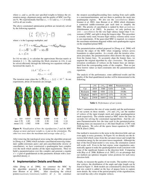
w 1 0.0 0.015 0.040 0.060 0.10 0.7
max 3.70 1.82 1.98 2.30 2.46 1.14
mean 3.32 1.502 0.98 0.84 0.67 0.23
Figure 9: Visualization of how the eigenfunction f and the MSC
change as more and more weight w 1 is put on the orientation. The
other two rows show the maximum and average value of c 2 uv.
After removing the topological noise using the algorithm proposed
in [Dong et al. 2006] which includes cancellation(removing redundant
saddle-extremum pairs) and anti-cancellation(the inverse of
cancellation), we have constructed a quadrangular base complex
over the mesh which satisfies all the input requirements. Then we
build a parameterization over this complex and generate a regular
d × d grid of quadrilaterals in this parametric domain with a userspecified
density d.
4 Implementation Details and Results
Alike [Dong et al. 2006], we construct the MSC by
the algorithm proposed in [Edelsbrunner et al. 2003;
timo Bremer et al. 2004]. After classifying the critical
points(maximum/minimum/saddle) of f, we construct
Tabel 1 summarizes the size of some models and the performance
of our system on these models. |M| and |M q| are the number
of vertices of the input triangle mesh and output quadrangulation
mesh respectively. The column named as MSC shows the time (in
seconds) for solving the constrained eigenproblem. And the column
Parameterization lists the time used in the parameterization.
Running times are measured on a 1.8G Intel DualCore 2 CPU with
2GB memory. We solve all the sparse linear equations by UMF-
PACK [Davis 2004].
Our method is insensitive to the noise in the direction field, and can
even apply to noisy geometry. In Figure 10, we directly use the direction
field which comes from the curvature tensor and weight the
orientation energy by the curvature tensor magnitude. Although the
hair of the David head model is very noisy, the orientation control
still works well. Even in the hair region, some singularities automatically
appear to make the quadrangulation result consistent with
some of the significant features in the direction field. Comparing
with [Ray et al. 2006; Kälberer et al. 2007], it’s an advantage that
our method can optimize irregular vertex positions for such noisy
direction field.
Finally, we measure the quality of our results. The number of irregular
vertices, the distribution of the angle and edge length can be
found in Figure 11. Both models are constrained by direction field,
and size control is added on the face of pegaso horse to capture
more details. By virtue of the period property of the eigenfunction,
our result has only a few irregular vertices.