Efficient Simplification of Point-Sampled Surfaces - Computer ...

Efficient Simplification of Point-Sampled Surfaces
Mark Pauly Markus Gross Leif P. Kobbelt
ETH Zürich ETH Zürich RWTH Aachen
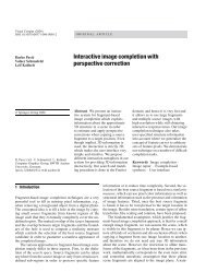
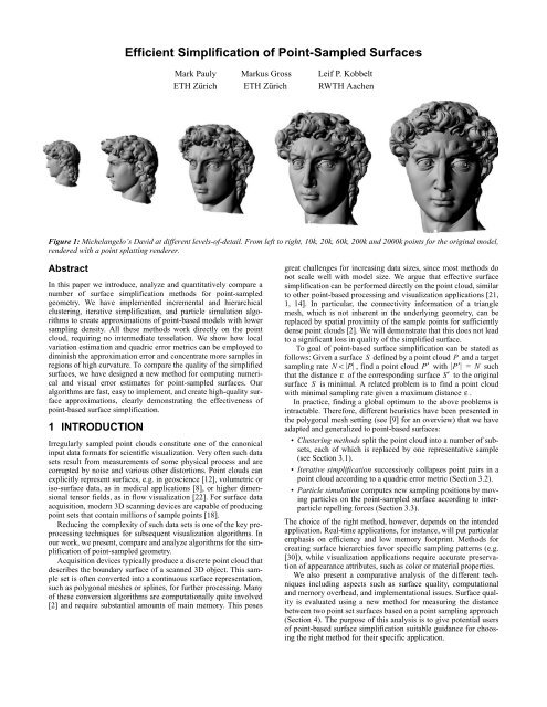
Figure 1: Michelangelo’s David at different levels-of-detail. From left to right, 10k, 20k, 60k, 200k and 2000k points for the original model,
rendered with a point splatting renderer.
Abstract
In this paper we introduce, analyze and quantitatively compare a
number of surface simplification methods for point-sampled
geometry. We have implemented incremental and hierarchical
clustering, iterative simplification, and particle simulation algorithms
to create approximations of point-based models with lower
sampling density. All these methods work directly on the point
cloud, requiring no intermediate tesselation. We show how local
variation estimation and quadric error metrics can be employed to
diminish the approximation error and concentrate more samples in
regions of high curvature. To compare the quality of the simplified
surfaces, we have designed a new method for computing numerical
and visual error estimates for point-sampled surfaces. Our
algorithms are fast, easy to implement, and create high-quality surface
approximations, clearly demonstrating the effectiveness of
point-based surface simplification.
1 INTRODUCTION
Irregularly sampled point clouds constitute one of the canonical
input data formats for scientific visualization. Very often such data
sets result from measurements of some physical process and are
corrupted by noise and various other distortions. Point clouds can
explicitly represent surfaces, e.g. in geoscience [12], volumetric or
iso-surface data, as in medical applications [8], or higher dimensional
tensor fields, as in flow visualization [22]. For surface data
acquisition, modern 3D scanning devices are capable of producing
point sets that contain millions of sample points [18].
Reducing the complexity of such data sets is one of the key preprocessing
techniques for subsequent visualization algorithms. In
our work, we present, compare and analyze algorithms for the simplification
of point-sampled geometry.
Acquisition devices typically produce a discrete point cloud that
describes the boundary surface of a scanned 3D object. This sample
set is often converted into a continuous surface representation,
such as polygonal meshes or splines, for further processing. Many
of these conversion algorithms are computationally quite involved
[2] and require substantial amounts of main memory. This poses
great challenges for increasing data sizes, since most methods do
not scale well with model size. We argue that effective surface
simplification can be performed directly on the point cloud, similar
to other point-based processing and visualization applications [21,
1, 14]. In particular, the connectivity information of a triangle
mesh, which is not inherent in the underlying geometry, can be
replaced by spatial proximity of the sample points for sufficiently
dense point clouds [2]. We will demonstrate that this does not lead
to a significant loss in quality of the simplified surface.
To goal of point-based surface simplification can be stated as
follows: Given a surface S defined by a point cloud P and a target
sampling rate N < P , find a point cloud P′ with P′ = N such
that the distance ε of the corresponding surface S′ to the original
surface S is minimal. A related problem is to find a point cloud
with minimal sampling rate given a maximum distance ε .
In practice, finding a global optimum to the above problems is
intractable. Therefore, different heuristics have been presented in
the polygonal mesh setting (see [9] for an overview) that we have
adapted and generalized to point-based surfaces:
• Clustering methods split the point cloud into a number of subsets,
each of which is replaced by one representative sample
(see Section 3.1).
• Iterative simplification successively collapses point pairs in a
point cloud according to a quadric error metric (Section 3.2).
• Particle simulation computes new sampling positions by moving
particles on the point-sampled surface according to interparticle
repelling forces (Section 3.3).
The choice of the right method, however, depends on the intended
application. Real-time applications, for instance, will put particular
emphasis on efficiency and low memory footprint. Methods for
creating surface hierarchies favor specific sampling patterns (e.g.
[30]), while visualization applications require accurate preservation
of appearance attributes, such as color or material properties.
We also present a comparative analysis of the different techniques
including aspects such as surface quality, computational
and memory overhead, and implementational issues. Surface quality
is evaluated using a new method for measuring the distance
between two point set surfaces based on a point sampling approach
(Section 4). The purpose of this analysis is to give potential users
of point-based surface simplification suitable guidance for choosing
the right method for their specific application.

Earlier methods for simplification of point-sampled models
have been introduced by Alexa et al. [1] and Linsen [20]. These
algorithms create a simplified point cloud that is a true subset of
the original point set, by ordering iterative point removal operations
according to a surface error metric. While both papers report
good results for reducing redundancy in point sets, pure subsampling
unnecessarily restricts potential sampling positions, which
can lead to aliasing artefacts and uneven sampling distributions. To
alleviate these problems, the algorithms described in this paper
resample the input surface and implicitly apply a low-pass filter
(e.g. clustering methods perform a local averaging step to compute
the cluster’s centroid).
In [21], Pauly and Gross introduced a resampling strategy based
on Fourier theory. They split the model surface into a set of
patches that are resampled individually using a spectral decomposition.
This method directly applies signal processing theory to
point-sampled geometry, yielding a fast and versatile point cloud
decimation method. Potential problems arise due to the dependency
on the specific patch layout and difficulties in controlling
the target model size by specifying spectral error bounds.
Depending on the intended application, working directly on the
point cloud that represents the surface to be simplified offers a
number of advantages:
• Apart from geometric inaccuracies, noise present in physical
data can also lead to topological distortions, e.g. erroneous
handles or loops, which cause many topology-preserving simplification
algorithms to produce inferior results (see [32], Figure
3). Point-based simplification does not consider local
topology and is thus not affected by these problems. If topological
invariance is required, however, point-based simplification
is not appropriate.
• Point-based simplification can significantly increase performance
when creating coarse polygonal approximations of
large point sets. Instead of using a costly surface reconstruction
for a detailed point cloud followed by mesh simplification,
we first simplify the point cloud and only apply the
surface reconstruction for the much smaller, simplified point
set. This reconstruction will also be more robust, since geometric
and topological noise is removed during the point-based
simplification process.
• Upcoming point-based visualization methods [14, 25, 23] can
benefit from the presented simplification algorithms as different
level-of-detail approximations can be directly computed
from their inherent data structures.
• The algorithms described in this paper are time and memory
efficient and easy to implement. Unlike triangle simplification,
no complex mesh data structures have to be build and maintained
during the simplification, leading to an increased overall
performance.
We should note that our algorithms are targeted towards denselysampled
organic shapes stemming from 3D acquisition, iso-surface
extraction or sampling of implicit functions. They are not
suited for surfaces that have been carefully designed in a particular
surface representation, such as low-resolution polygonal CAD
data. Also our goal is to design algorithms that are general in the
sense that they do not require any knowledge of the specific source
of the data. For certain applications this additional knowledge
could be exploited to design a more effective simplification algorithm,
but this would also limit the applicability of the method.
2 LOCAL SURFACE PROPERTIES
In this section we describe how we estimate local surface properties
from the underlying point cloud. These techniques will be used
in the simplification algorithms presented below: Iterative simplification
(Section 3.2) requires an accurate estimation of the tangent
plane, while clustering (Section 3.1) employs a surface variation
estimate (Section 2.1). Particle simulation (Section 3.3) makes use
of both methods and additionally applies a moving least-squares
projection operator (Section 2.2) that will also be used for measuring
surfaces error in Section 4.
Our algorithms take as input an unstructured point cloud
P = { p i
∈ IR 3 } describing a smooth, two-manifold boundary
surface S of a 3D object. The computations of local surface properties
are based on local neighborhoods of sample points. We
found that the set of k -nearest neighbors of a sample p ∈ P ,
denoted by the index set N p , works well for all our models. More
sophisticated neighborhoods, e.g. Floater’s method based on local
Delaunay triangulations [5] or Linsen’s angle criterion [20] could
be used for highly non-uniformly sampled models at the expense
of higher computational overhead. To obtain an estimate of the
local sampling density ρ at a point p , we define ρ = k⁄
r 2 ,
where r is the radius of the enclosing sphere of the k-nearest
neighbors of p given by r = max i ∈ Np
p – p i
.
2.1 Covariance Analysis
As has been demonstrated in earlier work (e.g. [11] and [27]),
eigenanalysis of the covariance matrix of a local neighborhood can
be used to estimate local surface properties. The 3×
3 covariance
matrix C for a sample point p is given by
C =
p i1
p ik
– p
…
– p
T
⋅
, (1)
where p is the centroid of the neighbors p ij
of p (see Figure 2).
Consider the eigenvector problem
C⋅ v l
= λ l
⋅ v l
, l ∈ { 012 , , }. (2)
Since C is symmetric and positive semi-definite, all eigenvalues
λ l
are real-valued and the eigenvectors v l
form an orthogonal
frame, corresponding to the principal components of the point set
defined by N p
[13]. The λ l
measure the variation of the
p i
, i ∈ N p
, along the direction of the corresponding eigenvectors.
The total variation, i.e. the sum of squared distances of the p i
from their center of gravity is given by
p
p i
2
∑
p i
– p = λ 0
+ λ 1
+ λ 2
. (3)
i ∈
r
N p
N p
(a)
(b)
Figure 2: Local neighborhood (a) and covariance analysis (b).
p i1
p ik
T( x)
– p
… ,
– p
Normal Estimation. Assuming λ 0
≤λ 1
≤λ 2
, it follows that
the plane
T( x): ( x–
p) ⋅ v 0
= 0
(4)
through p minimizes the sum of squared distances to the neighbors
of p [13]. Thus v 0
approximates the surface normal n p
at
p, or in other words, v 1
and v 2
span the tangent plane at p . To
compute a consistent orientation of the normal vectors, we use a
method based on the minimum spanning tree, as described in [11].
i j
λ 1
v 1
∈
N p
λ 0
v 0
p i
p
covariance ellipsoid

Clustering methods have been used in many computer graphics
applications to reduce the complexity of 3D objects. Rossignac
and Borrel, for example, used vertex clustering to obtain multiresolution
approximations of complex polygonal models for fast rendering
[24]. The standard strategy is to subdivide the model’s
bounding box into grid cells and replace all sample points that fall
into the same cell by a common representative. This volumetric
approach has some drawbacks, however. By using a grid of fixed
size this method cannot adapt to non-uniformities in the sampling
distribution. Furthermore, volumetric clustering easily joins
unconnected parts of a surface, if the grid cells are too large. To
alleviate these shortcomings, we use a surface-based clustering
approach, where clusters are build by collecting neighboring samples
while regarding local sampling density. We distinguish two
general approaches for building clusters. An incremental
approach, where clusters are created by region-growing, and a
hierarchical approach that splits the point cloud into smaller sub-
Surface Variation. λ 0
quantitatively describes the variation
along the surface normal, i.e. estimates how much the points deviate
from the tangent plane (4). We define
σ n
( p)
=
as the surface variation at point p in a neighborhood of size n . If
σ n
( p) = 0 , all points lie in the plane. The maximum surface variation
σ n
( p) = 1⁄
3 is assumed for completely isotropically distributed
points. Note that surface variation is not an intrinsic
feature of a point-sampled surface, but depends on the size of the
neighborhood. Note also that λ 1
and λ 2
describe the variation of
the sampling distribution in the tangent plane and can thus be used
to estimate local anisotropy.
Many surface simplification algorithms use curvature estimation
to decrease the error of the simplified surface by concentrating
more samples in regions of high curvature. As Figure 3 illustrates,
surface variation is closely related to curvature.
However, σ n
is more suitable for simplification
of point-sampled surfaces than cur-
N p
vature estimation based on function fitting.
p
Consider a surface with two opposing flat
parts that come close together. Even though a
low curvature would indicate that few sampling
points are required to adequately represent
the surface, for point-based surfaces we need a high sample
density to be able to distinguish the different parts of the surface.
This is more adequately captured by the variation measure .
2.2 Moving Least Squares Surfaces
Recently, Levin has introduced a new point-based surface representation
called moving least squares (MLS) surfaces [17]. Based
on this representation, Alexa et al. have implemented a high-quality
rendering algorithm for point set surfaces [1]. We will briefly
review the MLS projection operator and discuss an extension for
non-uniform sampling distributions.
Given a point set P, the MLS surface S MLS ( P)
is defined
implicitly by a projection operator Ψ as the points that project
onto themselves, i.e. S MLS ( P) = { x∈
IR 3 Ψ( P,
x)
= x}
.
Ψ( P,
r)
is defined by a two-step procedure: First a local reference
plane H = { x∈ IR 3 x⋅
n– D = 0}
is computed by minimizing
the weighted sum of squared distances
∑
p ∈ P
(5)
, (6)
where q is the projection of r onto H and h is a global scale factor.
Then a bivariate polynomial guv ( , ) is fitted to the points projected
onto the reference plane H using a similar weighted least
squares optimization. The projection of r onto S MLS
( P)
is then
given as Ψ( P,
r) = q + g( 00 , ) ⋅ n (for more details see [17, 1]).
Adaptive MLS Surfaces. Finding a suitable global scale factor
h can be difficult for non-uniformly sampled point clouds. In
regions of high sampling density many points need to be considered
in the least squares equations leading to high computational
cost. Even worse, if the sampling density is too low, only very few
points will contribute to Equation (6) due to the exponential falloff
of the weight function. This can cause instabilities in the optimization
which lead to wrong surface approximations. We propose
an extension of the static MLS approach, where instead of considering
samples within a fixed radius proportional to h , we collect
the k-nearest neighbors and adapt h according to the radius r of
the enclosing sphere. By dynamically choosing h = r⁄
3 , we
ensure that only points within the k -neighborhood contribute
noticeably to the least-squares optimization of Equation (6). While
λ 0
-----------------------------
λ 0
+ λ 1
+ λ 2
( p⋅
n–
D) 2 –
e r q
– 2 2
⁄ h
σ n
our experiments indicate that this adaptive scheme is more robust
than the standard method, a mathematical analysis of the implications
remains to be done.
(a) original surface
(c) variation σ 20 (d) variation σ 50
Figure 3: Comparison of surface curvature and surface variation
on the igea model (a). In (b), curvature is computed analytically
from a cubic polynomial patch fitted to the point set using moving
least squares (see Section 2.2). (c) and (d) show surface variation
for different neighborhood sizes.
3 SURFACE SIMPLIFICATION METHODS
In this section we present a number of simplification algorithms
for surfaces represented by discrete point clouds: Clustering methods
are fast and memory-efficient, iterative simplification puts
more emphasis on high surface quality, while particle simulation
allows intuitive control of the resulting sampling distribution.
After describing the technical details, we will discuss the specific
pros and cons of each method in more detail in Section 5.
3.1 Clustering
(b) mean curvature

p C
sets in a top-down manner [3, 27]. Both methods create a set { C i
}
of clusters, each of which is replaced by a representative sample,
typically its centroid, to create the simplified point cloud P′ .
Clustering by Region-growing. Starting from a random seed
point , a cluster is built by successively adding nearest
0 0
neighbors. This incremental region-growing is terminated when
the size of the cluster reaches a maximum bound. Additionally, we
can restrict the maximum allowed variation σ n
of each cluster.
This results in a curvature-adaptive clustering method, where more
and smaller clusters are created in regions of high surface variation.
The next cluster is then build by starting the incremental
C 1
growth with a new seed chosen from the neighbors of C 0
and
excluding all points of C 0
from the region-growing. Due to fragmentation,
this method creates many clusters that did not reach the
maximum size or variation bound, but whose incremental growth
was restricted by adjacent clusters. To obtain a more even distribution
of clusters, we distribute the sample points of all clusters that
did not reach a minimum size and variation bound (typically half
the values of the corresponding maximum bounds) to neighboring
clusters (see Figure 4 (a)). Note that this potentially increases the
size and variation of the clusters beyond the user-specified maxima.
Figure 5: Clustering: Uniform incremental clustering is shown in
The split plane is defined by the centroid of P and the eigenvector matrix Q v
. The quality of the collapse ( v 1
, v 2
) → v is then rated
v of the covariance matrix of with largest corresponding according to the minimum of the error functional
2
P
eigenvector (see Figure 2 (b)). Hence the point cloud is always Q v
= Q v1
+ Q v2
.
split along the direction of greatest variation (see also [3, 27]). If In order to adapt this technique to the decimation of unstructured
point clouds we use the k -nearest neighbor relation, since
the splitting criterion is not fulfilled, the point cloud P becomes a
cluster C i
. As shown in Figure 4 (b), hierarchical clustering builds manifold surface connectivity is not available. To initialize the
a binary tree, where each leaf of the tree corresponds to a cluster. A error quadrics for every point sample p , we estimate a tangent
straightforward extension to the recursive scheme uses a priority plane E i
for every edge that connects p with one of its neighbors
queue to order the splitting operations [3, 27]. While this leads to a p i
. This tangent plane is spanned by the vector e i
= p – p i
and
significant increase in computation time, it allows direct control b i
= e i
× n , where n is the estimated normal vector at p. After
over the number of generated samples, which is difficult to achieve this initialization the point cloud decimation works exactly like
by specifying n max
and σ max
only. Figure 5 illustrates both incremental
and hierarchical clustering, where we use oriented circular its ancestors p 1
mesh decimation with the point p inheriting the neighborhoods of
and p 2
and being assigned the error functional
splats to indicate the sampling distribution.
Q v
= Q v1
+ Q v2
. Figure 6 shows an example of a simplified point
cloud created by iterative point-pair contraction.
3.2 Iterative Simplification
3.3 Particle Simulation
A different strategy for point-based surface simplification iteratively
C 2
leaf node
split plane the left column, adaptive hierarchical clustering in the right column.
The top row illustrates the clusters on the original point set,
=cluster
the bottom row the resulting simplified point set (1000 points),
v 2 centroid
where the size of the splats corresponds to cluster size.
error metric that quantifies the error caused by the decimation. The
iteration is then performed in such a way that the decimation operation
causing the smallest error is applied first. Earlier work [1],
0 C 1
C
[20] uses simple point removal, i.e. points are iteratively removed
(a)
(b)
from the point cloud, resulting in a simplified point cloud that is a
Figure 4: (a) Clustering by incremental region growing, where
“stray samples” (black dots) are attached to the cluster with closest
centroid. (b) Hierarchical clustering, where the thickness of the
lines indicates the level of the BSP tree (2D for illustration).
subset of the original point set. As discussed above, true subsampling
is prone to aliasing and often creates uneven sampling distributions.
Therefore, we use point-pair contraction, an extension of
the common edge collapse operator, which replaces two points p 1
and p 2
by a new point p . To rate the contraction operation, we
Hierarchical Clustering. A different method for computing use an adaptation of the quadric error metric presented for polygonal
the set of clusters recursively splits the point cloud using a binary
space partition. The point cloud P is split if:
meshes in [6]. The idea here is to approximate the surface
locally by a set of tangent planes and to estimate the geometric
• The size P is larger than the user specified maximum cluster
deviation of a mesh vertex v from the surface by the sum of the
size n or
squared distances to these planes. The error quadrics for each vertex
v are initialized with a set of planes defined by the triangles
max
• the variation σ n
( P) is above a maximum threshold σ max
. around that vertex and can be represented by a symmetric 4×
4
reduces the number of points using an atomic decimation
operator. This approach is very similar to mesh-based simplification
methods for creating progressive meshes [10]. Decimation
operations are usually arranged in a priority queue according to an
In [29], Turk introduced a method for resampling polygonal surfaces
using particle simulation. The desired number of particles is
randomly spread across the surface and their position is equalized
using a point repulsion algorithm. Point movement is restricted to

p is kept on the surface by simply projecting it onto the tangent
plane of the point p′ of the original point cloud that is closest to
p . Only at the end of the simulation, we apply the full moving
least squares projection, which alters the particle positions only
slightly and does not change the sampling distribution noticeably.
Adaptive Simulation. Using the variation estimate of Section
2.1, we can concentrate more points in regions of high curvature
by scaling their repulsion radius with the inverse of the variation
σ n
. It is also important to adapt the initial spreading of particles
accordingly to ensure fast convergence. This can be done by
replacing the density estimate ρ by ρ ⋅ σ n
. Figure 7 gives an
example of an adaptive particle simulation.
Figure 6: Iterative simplification of the Isis model from 187,664
(left) to 1,000 sample points (middle). The right image shows all remaining
potential point-pair contractions indicated as an edge between
two points. Note that these edges do not necessarily form a
consistent triangulation of the surface.
the surface defined by the individual polygons to ensure an accurate
approximation of the original surface. Turk also included a
curvature estimation method to concentrate more samples in
regions of high curvature. Finally, the new vertices are re-triangulated
yielding the resampled triangle mesh. This scheme can easily
be adapted to point-sampled geometry.
Spreading Particles. Turk initializes the particle simulation
by randomly distributing points on the surface. Since a uniform
initial distribution is crucial for fast convergence, this random
choice is weighted according to the area of the polygons. For
point-based models, we can replace this area measure by a density
estimate ρ (see Section 2). Thus by placing more samples in
regions of lower sampling density (which correspond to large triangles
in the polygonal setting), uniformity of the initial sample
distribution can ensured.
Repulsion. We use the same linear repulsion force as in [29],
because its radius of influence is finite, i.e. the force vectors can be
computed very efficiently as
F i
( p) = kr ( – p – p i
) ⋅ ( p – p i
), (7)
where F i
( p) is the force exerted on particle p due to particle p i
,
k is a force constant and r is the repulsion radius. The total force
exertedonp
isthengivenas
∑
F( p) = F i
( p)
, (8)
i∈
where N p
is the neighborhood of p with radius r . Using a 3D
grid data structure, this neighborhood can be computed efficiently
in constant time.
Projection. In Turk’s method, displaced particles are projected
onto the closest triangle to prevent to particles from drifting away
from the surface. Since we have no explicit surface representation
available, we use the MLS projection operator Ψ (see Section 2.2)
to keep the particles on the surface. However, applying this projection
every time a particle position is altered is computationally too
expensive. Therefore, we opted for a different approach: A particle
N p
Figure 7: Simplification by adaptive particle simulation. The left
image shows the original model consisting of 75,781 sample points.
On the right, a simplified version consisting of 6,000 points is
shown, where the size of the splats is proportional to the repelling
force of the corresponding particle.
4 ERROR MEASUREMENT
In Section 3 we have introduced different algorithms for pointbased
surface simplification. To evaluate the quality of the surfaces
generated by these methods we need some means for measuring
the distance between two point-sampled surfaces. Our goal
is to give both numerical and visual error estimates, without
requiring any knowledge about the specific simplification algorithm
used. In fact, our method can be applied to any pair of pointsampled
surfaces. Assume we have two point clouds P and P′
representing two surfaces S and S′ , respectively. Similar to the
Metro tool [4], we use a sampling approach to approximate surface
error. We measure both the maximum error ∆ max
( SS′ , ), i.e. the
two-sided Hausdorff distance, and the mean error ∆ avg
( SS′ , ), i.e.
the area-weighted integral of the point-to-surfaces distances. The
idea is to create an upsampled point cloud Q of points on S and
compute the distance d( q,
S′ ) = min p′ ∈ S′
d( qp′ , ) for each
q ∈ Q .Then
∆ max
( SS′ , ) ≈ max q ∈ Q
d( q,
S′ ) and (9)
1
∆ avg
( SS′ , ) ≈ ------ d( q,
S′ ). (10)
Q ∑
q ∈ Q
d( q,
S′ ) is calculated using the MLS projection operator Ψ with
linear basis function (see Section 2.2). Effectively, Ψ computes
the closest point q′ ∈ S′ such that q = q′ + d ⋅ n for a q ∈ Q ,
where n is the surface normal at q′ and d is the distance between
q and q′ (see Figure 8). Thus the point-to-surface distance
d( q,
S′ ) is given as d = qq′ . Note that this surface-based
approach is crucial for meaningful error estimates, as the Haussdorff
distance of the two point sets P and P′ does not adequately
measure the distance between S and S′ . As an example, consider

a point cloud P′ that has been created by randomly subsampling
P . Even though the corresponding surfaces can be very different,
the Haussdorff distance of the point sets will always be zero.
To create the upsampled point cloud Q we use the uniform particle
simulation of Section 3.3. This allows the user to control the
accuracy of the estimates (9) and (10) by specifying the number of
points in Q . To obtain a visual error estimate, the sample points of
Q can be color-coded according to the point-to-surface distance
dqS′ ( , ) and rendered using a standard point rendering technique
(see Figures 10 and 13).
S
S′
q ∈ Q
p′ ∈ P′
p ∈ P
Figure 8: Measuring the distance between two surfaces S (red
curve) and S′ (black curve) represented by two point sets P (red
dots) and P′ (black dots). P is upsampled to Q (blue dots) and for
each q ∈ Q a base point q′ ∈ S′ is found (green dots), such that
the vector qq′ is orthogonal to S′ . The point-to-surface distance
d( q,
S′ ) is then equal to d = qq′ .
5 RESULTS & DISCUSSION
}
q′
We have implemented the algorithms described in Section 3 and
conducted a comparative analysis using a large set of point-sampled
models. We also examined smoothing effects of the simplification
and MLS projection (Section 5.2) and compared pointbased
simplification with mesh-based simplification (Section 5.3).
5.1 Comparison of Simplification Methods
Surface error has been measured using the method presented in
Section 4. Additionally, we considered aspects such as sampling
distribution of the simplified model, time and space efficiency and
implementational issues. For conciseness, Figures 9 (a) and 10
show evaluation data for selected models that we found representative
for a wide class of complex point-based surfaces.
Surface Error. Figure 10 shows visual and quantitative error
estimates (scaled according to the object’s bounding box diagonal)
for the David model that has been simplified from 2,000,606
points to 5,000 points (see also Figure 1). Uniform incremental
clustering has the highest average error and since all clusters consist
of roughly the same number of sample points, most of the error
is concentrated in regions of high curvature. Adaptive hierarchical
clustering performs slightly better, in particular in the geometrically
complex regions of the hair. Iterative simplification and particle
simulation provide lower average error and distribute the error
more evenly across the surface. In general we found the iterative
simplification method using quadric error metrics to produce the
lowest average surface error.
Sampling Distribution. For clustering methods the distribution
of samples in the final model is closely linked to the sampling
distribution of the input model. In some applications this might be
desirable, e.g. where the initial sampling pattern carries some
semantics such as in geological models. Other applications, e.g.
pyramid algorithms for multilevel smoothing [15] or texture synthesis
[30], require uniform sampling distributions, even for highly
non-uniformly sampled input models. Here non-adaptive particle
simulation is most suitable, as it distributes sample points uniformly
and independent of the sampling distribution of the underlying
surface. As illustrated in Figure 11, particle simulation also
q
d
provides a very easy mechanism for locally controlling the sampling
density by scaling the repulsion radius accordingly. While
similar effects can be achieved for iterative simplification by
penalizing certain point-pair contractions, we found that particle
simulation offers much more intuitive control. Also note the
smooth transition in sampling rate shown in the zoomed region.
Computational Effort. Figure 9 shows computation times for
the different simplification methods both as a function of target
model size and input model size. Due to the simple algorithmic
structure, clustering methods are by far the fastest technique presented
in this paper. Iterative simplification has a relatively long
pre-computing phase, where initial contraction candidates and corresponding
error quadrics are determined and the priority queue is
set up. The simple additive update rule of the quadric metric (see
Section 3.2) make the simplification itself very efficient, however.
In our current implementation particle simulation is the slowest
simplification technique for large target model sizes, mainly due to
slow convergence of the relaxation step. We believe, however, that
this convergence can be improved considerably by using a hierarchical
approach similar to [31]. The algorithm would start with a
small number of particles and relax until the particle positions
have reached equilibrium. Then particles are split, their repulsion
radius is adapted and relaxation continues. This scheme can be
repeated until the desired number of particles is obtained.
It is interesting to note that for incremental clustering and iterative
simplification the execution time increases with decreasing
target model size, while hierarchical clustering and particle simulation
are more efficient the smaller the target models. Thus the
latter are more suitable for real-time applications where the fast
creation of coarse model approximations is crucial.
70
60
50
40
30
20
10
Execution time (secs.)
0
180
160
140
120
100
Execution time (secs.)
500
Incremental Clustering
450
Hierarchical Clustering
400
350
300
250
200
150
100
50
0
Santa
Igea
Isis
Iterative Simplification
Particle Simulation
Dragon
(a)
(b)
Figure 9: Execution times for simplification, measured on a Pentium
4 (1.8GHz) with 1Gb of main memory: (a) as a function of target
model size for the dragon model (435,545 points), (b) as a
function of input model size for a simplification to 1%.
80
David
Incremental Clustering
Hierarchical Clustering
Iterative Simplification
Particle Simulation
60
40
20
simplified model size (*1000)
St.Matthew
0 500 1000 1500 2000 2500 3000 3500
input model size (*1000)
0

Memory Requirements and Data Structures. Currently all
methods presented in this paper are implemented in-core, i.e.
require the complete input model as well as the simplified point
cloud to reside in main memory. For incremental clustering we use
a balanced kd-tree for fast nearest-neighbor queries, which can be
implemented efficiently as an array [26] requiring 4 ⋅ N bytes,
where N is the size of the input model. Hierarchical clustering
builds a BSP tree, where each leaf node corresponds to a cluster.
Since the tree is build by re-ordering the sample points, each node
only needs to store the start and end index in the array of sample
points and no additional pointers are required. Thus this maximum
number of additional bytes is 2⋅ 2⋅4 ⋅M
, where M is the size of
the simplified model. Iterative simplification requires 96 bytes per
point contraction candidate, 80 of which are used for storing the
error quadric (we use doubles here as we found that single precision
floats lead to numerical instabilities). If we assume six initial
neighbors for each sample point, this amounts to 6⁄ 2 ⋅96 ⋅N
bytes. Particle simulation uses a 3D grid data structure with bucketing
to accelerate the nearest neighbor queries, since a static kdtree
is not suitable for dynamically changing particle positions.
This requires a maximum of 4 ⋅ ( N+
K)
bytes, where K is the
resolution of the grid.
Thus incremental clustering, iterative simplification and particle
simulation need additional storage that is linearly proportional to
the number of input points, while the storage overhead for hierarchical
clustering depends only on the target model size.
5.2 Simplification and Smoothing
Figure 12 demonstrates the smoothing effect of simplification in
connection with the MLS projection. The dragon has first been
simplified from 435,545 to 9,863 points using incremental clustering
and upsampled to its original size using particle simulation.
Observe the local shrinkage effects that also occur in iterative
Laplacian smoothing [28]. Computing the centroid of each cluster
is in fact very similar to a discrete approximation of the Laplacian.
Additionally, the MLS projection with Gaussian weight function
implicitly defines a Gaussian low-pass filter.
5.3 Comparison to Mesh Simplification
In Figure 13 we compare point-based simplification with simplification
for polygonal meshes. In (a), the initial point cloud is simplified
from 134,345 to 5,000 points using the iterative
simplification method of Section 3.2. The resulting point cloud has
then been triangulated using the surface reconstruction method of
[7]. In (b), we first triangulated the input point cloud and then simplified
the resulting polygonal surface using the mesh simplification
tool QSlim [6]. Both methods produce similar results in terms
of surface error and both simplification processes take approximately
the same time (~3.5 seconds). However, creating the trianglemeshfromthesimplifiedpointcloudtook2.45secondsin(a),
while in (b) reconstruction time for the input point cloud was 112.8
seconds. Thus when given a large unstructured point cloud, it is
much more efficient to first do the simplification on the point data
and then reconstruct a mesh (if desired) than to first apply a reconstruction
method and then simplify the triangulated surface. This
illustrates that our methods can be very useful when dealing with
large geometric models stemming from 3D acquisition.
6 CONCLUSIONS & FUTURE WORK
We have presented and analyzed different strategies for surface
simplification of geometric models represented by unstructured
point clouds. Our methods are fast, robust and create surfaces of
high quality, without requiring a tesselation of the underlying surface.
We have also introduced a versatile tool for measuring the
distance between two point-sampled surfaces. We believe that the
surface simplification algorithms presented in this paper can be the
basis of many point-based processing applications such as multilevel
smoothing, multiresolution modeling, compression, and efficient
level-of-detail rendering.
Directions for future work include out-of-core implementations
of the presented simplification methods, design of appearance-preserving
simplification, progressive schemes for representing pointbased
surface and point-based feature extraction using the variation
estimate σ n
.
Acknowledgements
Our thanks to Marc Levoy and the Digital Michelangelo Project
people for making their models available to us. This work is supported
by the joint Berlin/Zurich graduate program Combinatorics,
Geometry, and Computation, financed by ETH Zurich and the German
Science Foundation (DFG).
References
[1] Alexa, M., Behr, J., Cohen-Or, D., Fleishman, S., Levin, D., Silva, T. Point
Set Surfaces, IEEE Visualization 01, 2001
[2] Amenta, N., Bern, M., Kamvysselis, M. A New Voronoi-Based Surface
Reconstruction Algorithm. SIGGRAPH 98, 1998
[3] Brodsky, D., Watson, B. Model simplification through refinement. Proceedings
of Graphics Interface 2000,2000
[4] Cignoni, P., Rocchini, C., Scopigno, R. Metro: Measuring error on simplified
surfaces. Computer Graphics Forum, 17(2), June 1998
[5] Floater, M., Reimers, M. Meshless parameterization and surface reconstruction.
Comp. Aided Geom. Design 18, 2001
[6] Garland, M., Heckbert, P. Surface simplification using quadric error metrics.
SIGGRAPH 97,1997
[7] Giessen, J., John, M. Surface reconstruction based on a dynamical system.
EUROGRAPHICS 2002, to appear
[8] Gross, M. Graphics in Medicine: From Visualization to Surgery. ACM
Computer Graphics, Vol. 32, 1998
[9] Heckbert, P., Garland, M. Survey of Polygonal Surface Simplification
Algorithms. Multiresolution Surface Modeling Course. SIGGRAPH 97
[10] Hoppe, H. Progressive Meshes. SIGGRAPH 96, 1996
[11] Hoppe, H., DeRose, T., Duchamp, T., McDonald, J., Stuetzle, W. Surface
reconstruction from unorganized points. SIGGRAPH 92, 1992
[12] Hubeli, A., Gross, M. Fairing of Non-Manifolds for Visualization. IEEE
Visualization 00, 2000.
[13] Jolliffe, I. Principle Component Analysis. Springer-Verlag, 1986
[14] Kalaiah, A., Varshney, A. Differential Point Rendering. Rendering Techniques
01, Springer Verlag, 2001.
[15] Kobbelt, L., Campagna, S., Vorsatz, J., Seidel, H. Interactive Multi-Resolution
Modeling on Arbitrary Meshes. SIGGRAPH 98, 1998
[16] Kobbelt, L. Botsch, M., Schwanecke, U., Seidel, H. Feature Sensitive Surface
Extraction from Volume Data. SIGGRAPH 01, 2001
[17] Levin, D. Mesh-independent surface interpolation. Advances in Computational
Mathematics, 2001
[18] Levoy, M., Pulli, K., Curless, B., Rusinkiewicz, S., Koller, D., Pereira, L.,
Ginzton, M., Anderson, S., Davis, J., Ginsberg, J., Shade, J., Fulk, D. The
Digital Michelangelo Project: 3D Scanning of Large Statues. SIGGRAPH
00, 2000
[19] Lindstrom, P., Silva, C. A memory insensitive technique for large model
simplification. IEEE Visualization 01, 2001
[20] Linsen, L. Point Cloud Representation. Technical Report, Faculty of Computer
Science, University of Karlsruhe, 2001
[21] Pauly, M., Gross, M. Spectral Processing of Point-Sampled Geometry,
SIGGRAPH 01, 2001
[22] Peikert, R., Roth, M. The “Parallel Vectors” Operator - A Vector Field
Visualization Primitive. IEEE Visualization 99, 1999
[23] Pfister, H., Zwicker, M., van Baar, J., Gross, M. Surfels: Surface Elements
as Rendering Primitives. SIGGRAPH 00,2000
[24] Rossignac, J., Borrel, P. Multiresolution 3D approximations for rendering
complex scenes. Modeling in Computer Graphics: Methods and Applications,
1993
[25] Rusinkiewicz, S., Levoy, M. QSplat: A Multiresolution Point Rendering
System for Large Meshes. SIGGRAPH 00, 2000
[26] Sedgewick, R. Algorithms in C++ (3rd edition). Addison Wesley, 1998
[27] Shaffer, E., Garland, M. Efficient Adaptive Simplification of Massive
Meshes. IEEE Visualization 01, 2001
[28] Taubin, G. A Signal Processing Approach to Fair Surface Design. SIG-
GRAPH 95, 1995
[29] Turk, G. Re-Tiling Polygonal Surfaces. SIGGRPAH 92,1992
[30] Turk, G. Texture Synthesis on Surfaces. SIGGRAPH 01, 2001
[31] Witkin, A., Heckbert, P. Using Particles To Sample and Control Implicit
Surfaces. SIGGRAPH 94, 1994
[32] Wood, Z., Hoppe, H. Desbrun, M., Schröder, P. Isosurface Topology Simplification.,
see http://www.multires.caltech.edu/pubs/topo_filt.pdf

∆ max = 0.0049 ∆ avg = 6.32 ⋅ 10 – 4
∆ max = 0.0046 ∆ avg = 6.14 ⋅ 10 – 4
∆ max = 0.0052 ∆ avg = 5.43 ⋅ 10 – 4
∆ max = 0.0061 ∆ avg = 5.69 ⋅ 10 – 4
(a) uniform incremental clustering (b) adaptive hierarchical clustering (c) iterative simplification (d) particle simulation
Figure 10: Surface Error for Michelangelo’s David simplified from 2,000,606 points to 5,000 points.
original: 3,382,866 points
simplified: 30,000 points
Figure 11: User-controlled particle simulation. The repulsion radius has been decreased to 10% in the region marked by the blue circle.
(a) original: 435,545 points (b) simplified: 9,863 points (incremental clustering) (c) upsampled: 435,545 points (part. simulation)
Figure 12: Smoothing effect on the dragon by simplification and successive upsampling.
∆ max = 0.0011 ∆ avg = 5.58 ⋅ 10 – 5
∆ max = 0.0012 ∆ avg = 5.56 ⋅ 10 – 5
(a) Iterative point cloud simplification
(b) QSlim (mesh simplification)
Figure 13: Comparison between point cloud simplification and mesh simplification: The igea model simplified from 134,345 to 5,000 points.