sqrt(3) subdivision - Computer Graphics Group at RWTH Aachen

3-Subdivision
Leif Kobbelt¡
Max-Planck Institute for Computer Sciences
Abstract
A new stationary subdivision scheme is presented which performs
slower topological refinement than the usual dyadic split operation.
The number of triangles increases in every step by a factor of 3
instead of 4. Applying the subdivision operator twice causes a uniform
refinement with tri-section of every original edge (hence the
name ¢ 3-subdivision) while two dyadic splits would quad-sect every
original edge. Besides the finer gradation of the hierarchy levels,
the new scheme has several important properties: The stencils
for the subdivision rules have minimum size and maximum symmetry.
The smoothness of the limit surface is C 2 everywhere except for
the extraordinary points where it is C 1 . The convergence analysis
of the scheme is presented based on a new general technique which
also applies to the analysis of other subdivision schemes. The new
splitting operation enables locally adaptive refinement under builtin
preservation of the mesh consistency without temporary crackfixing
between neighboring faces from different refinement levels.
The size of the surrounding mesh area which is affected by selective
refinement is smaller than for the dyadic split operation. We
further present a simple extension of the new subdivision scheme
which makes it applicable to meshes with boundary and allows us
to generate sharp feature lines.
1 Introduction
The use of subdivision schemes for the efficient generation of
freefrom surfaces has become commonplace in a variety of geometric
modeling applications. Instead of defining a parameteric
surface by a functional expression F£ u¤ v¥ to be evaluated over a
planar parameter domain Ω ¦ IR 2 we simply sketch the surface by
a coarse control mesh M 0 that may have arbitrary connectivity and
(manifold) topology. By applying a set of refinement rules, we generate
a sequence of finer and finer meshes M 1 ¤¨§¨§©§¨¤ M k ¤¨§¨§¨§ which
eventually converge to a smooth limit surface M ∞ .
In the literature there have been proposed many subdivision
schemes which are either generalized from tensor-products of curve
generation schemes [DS78, CC78, Kob96] or from 2-scale relations
in more general functional spaces being defined over the threedirectional
grid [Loo87, DGL90, ZSS96]. Due to the nature of the
refinement operators, the generalized tensor-product schemes natu-
Max-Planck Institute for Computer Sciences, Im Stadtwald,
66123 Saarbrücken, Germany, kobbelt@mpi-sb.mpg.de
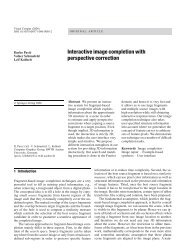
Figure 1: Subdivision schemes on triangle meshes are usually based
on the 1-to-4 split operation which inserts a new vertex for every
edge of the given mesh and then connects the new vertices.
rally lead to quadrilateral meshes while the others lead to triangle
meshes.
A subdivision operator for polygonal meshes can be considered
as being composed by a (topological) split operation followed by
a (geometric) smoothing operation. The split operation performs
the actual refinement by introducing new vertices and the smoothing
operation changes the vertex positions by computing averages
of neighboring vertices (generalized convolution operators, relaxation).
In order to guarantee that the subdivision process will always
generate a sequence of meshes M k that converges to a smooth
limit, the smoothing operator has to satisfy specific necessary and
sufficient conditions [CDM91, Dyn91, Rei95, Zor97, Pra98]. This
is why special attention has been paid by many authors to the design
of optimal smoothing rules and their analysis.
While in the context of quad-meshes several different topological
split operations (e.g. primal [CC78, Kob96] or dual [DS78])
have been investigated, all currently proposed stationary schemes
for triangle meshes are based on the uniform 1-to-4 split [Loo87,
DGL90, ZSS96] which is depicted in Fig 1. This split operation
introduces a new vertex for each edge of the given mesh.
Recently, the concept of uniform refinement has been generalized
to irregular refinement [GSS99, KCVS98, VG99] where new
vertices can be inserted at arbitrary locations without necessarily
generating semi-uniform meshes with so-called subdivision connectivity.
However, the convergence analysis of such schemes is
still an open question.
In this paper we will present a new subdivision scheme for triangle
meshes which is based on an alternative uniform split operator
that introduces a new vertex for every triangle of the given mesh
(Section 2).
As we will see in the following sections, the new split operator
enables us to define a natural stationary subdivision scheme which
has stencils of minimum size and maximum symmetry (Section 3).
The smoothing rules of the subdivision operator are derived from
well-known necessary conditions for the convergence to smooth
limit surfaces. Since the standard subdivision analysis machinery
cannot be applied directly to the new scheme, we derive a modified
technique and prove that the scheme generates C 2 surfaces for
regular control meshes. For arbitrary control meshes we find the
limit surface to be C 2 almost everywhere except for the extraordinary
vertices (valence 6) where the smoothness is at least C 1 (see
the Appendix).

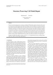
Figure 2: The ¢ 3-subdivision scheme is based on a split operation which first inserts a new vertex for every face of the given mesh. Flipping
the original edges then yields the final result which is a 30 degree rotated regular mesh. Applying the ¢ 3-subdivision scheme twice leads to
a 1-to-9 refinement of the original mesh. As this corresponds to a tri-adic split (two new vertices are introduced for every original edge) we
call our scheme ¢ 3-subdivision.
Inserting a new vertex into a triangular face does only affect that
single face which makes locally adaptive refinement very effective.
The global consistency of the mesh is preserved automatically if
¢ 3-subdivision is performed selectively. In Section 4 we compare
adaptively refined meshes generated by dyadic subdivision with our
¢ 3-subdivision meshes and find that ¢ 3-subdivision usually needs
fewer triangles and less effort to achieve the same approximation
tolerance. The reason for this effect is the better localization, i.e.,
only a relatively small region of the mesh is affected if more vertices
are inserted locally.
For the generation of surfaces with smooth boundary curves, we
need special smoothing rules at the boundary faces of the given
mesh. In Section 5 we propose a boundary rule which reproduces
cubic B-splines. The boundary rules can also be used to generate
sharp feature lines in the interior of the surface.
2 3-Subdivision
The most wide-spread way to uniformly refine a given triangle
mesh M 0 is the dyadic split which bi-sects all the edges by inserting
a new vertex between every adjacent pair of old ones. Each
triangular face is then split into four smaller triangles by mutually
connecting the new vertices sitting on a face’s edges (cf. Fig. 1).
This type of splitting has the positive effect that all newly inserted
vertices have valence six and the valences of the old vertices does
not change. After applying the dyadic split several times, the refined
meshes M k have a semi-regular structure since the repeated
1-to-4 refinement replaces every triangle of the original mesh by a
regular patch with 4 k triangles.
A straightforward generalization of the dyadic split is the n-adic
split where every edge is subdivided into n segments and consequently
every original face is split into n 2 sub-triangles. However,
in the context of stationary subdivision schemes, the n-adic split
operation requires a specific smoothing rule for every new vertex
(modulo permutations of the barycentric coordinates). This is why
subdivision schemes are mostly based on the dyadic split that only
requires two smoothing rules: one for the old vertices and one for
the new ones (plus rotations).
In this paper, we consider the following refinement operation for
triangle meshes: Given a mesh M 0 we perform a 1-to-3 split for
every triangle by inserting a new vertex at its center. This introduces
three new edges connecting the new vertex to the surrounding old
ones. In order to re-balance the valence of the mesh vertices we then
flip every original edge that connects two old vertices (cf. Fig 2).
This split operation is uniform in the sense that if it is applied to
a uniform (three-directional) grid, a (rotated and refined) uniform
grid is generated (cf. Fig. 2). If we apply the same refinement operator
twice, the combined operator splits every original triangle into
nine subtriangles (tri-adic split). Hence one single refinement step
can be considered as the ”square root” of the tri-adic split. In a different
context, this type of refinement operator has been considered
independently in [Sab87] and [Gus98].
Analyzing the action of ¢ the 3-subdivision operator on arbitrary
triangle meshes, we find that all newly inserted vertices have exactly
valence six. The valences of the old vertices are not changed
such that after a sufficient number of refinement steps, the mesh
M k has large regions with regular mesh structure which are disturbed
only by a small number of isolated extraordinary vertices.
These correspond to the vertices in M 0 which had valence 6 (cf.
Fig. 3).
There are several arguments why it is interesting to investigate
this particular refinement operator. First, it is very natural to subdivide
triangular faces at their center rather than splitting all three
edges since the coefficients of the subsequent smoothing operator
can reflect the threefold symmetry of the three-directional grid.
Second, the ¢ 3-refinement is in some sense slower than the standard
refinement since the number of vertices (and faces) increases
by the factor of 3 instead of 4. As a consequence, we have more
levels of uniform resolution if a prescribed target complexity of
the mesh must not be exceeded. This is why similar uniform refinement
operators for quad-meshes have been used in numerical
applications such as multi-grid solvers for finite element analysis
[Hac85, GZZ93].
From the computer graphics point of view the ¢ 3-refinement
has the nice property that it enables a very simple implementation
of adaptive refinement strategies with no inconsistent intermediate
states as we will see in Section 4.
In the context of polygonal mesh based multiresolution representations
[ZSS96, KCVS98, GSS99], the ¢ 3-hierarchies can provide
an intuitive and robust way to encode the detail information since
the detail coefficients are assigned to (¡ faces tangent planes) instead
of vertices.
3 Stationary smoothing rules
To complete the definition of our new subdivision scheme, we have
to find the two smoothing rules, one for the placement of the newly
inserted vertices and one for the relaxation of the old ones. For the
sake of efficiency, our goal is to use the smallest possible stencils
while still generating high quality meshes.
There are well-known necessary and sufficient criteria which
tell whether a subdivision scheme S is convergent or not and what
smoothness properties the limit surface has. Such criteria check if
the eigenvalues of the subdivision matrix have a certain distribution
and if a local regular parameterization exists in the vicinity of every
vertex on the limit surface [CDM91, Dyn91, Rei95, Zor97, Pra98].

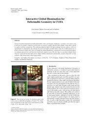
Figure 3: The ¢ 3-subdivision generates semi-regular meshes since all new vertices have valence six. After an even number 2k of refinement
steps, each original triangle is replaced by a regular patch with 9 k triangles.
By definition, the subdivision matrix is a square matrix S which
maps a certain sub-mesh V ¦ M k to a topologically equivalent submesh
S£ V¥ ¦ M k 1 of the refined mesh. Every row of this matrix is
a rule to compute the position of a new vertex. Every column of this
matrix tells how one old vertex contributes to the vertex positions
in the refined mesh. Usually, V is chosen to be the neighborhood of
a particular vertex, e.g., a vertex p and its neighbors up to the k-th
order (k-ring neighborhood).
To derive the weight coefficients for the new subdivision scheme,
we use these criteria for some kind of reverse engineering process,
i.e., instead of analyzing a given scheme, we derive one which by
construction satisifies the known necessary criteria. The justification
for doing this is that if the necessary conditions uniquely determine
a smoothing rule then the resulting subdivision scheme is the
only scheme (with the given stencil) that is worth being considered.
In the Appendix we will give the details of the sufficient part of the
convergence analysis.
Since the ¢ 3-subdivision operator inserts a new vertex for every
triangle of the given mesh, the minimum stencil for the corresponding
smoothing rule has to include at least the three (old) corner
vertices of that triangle. For symmetry reasons, the only reasonable
choice for that smoothing rule is hence
p
Figure 4: The application of the subdivision matrix S causes a rotation
around p since the neighboring vertices are replaced by the
centers of the adjacent triangles.
u v v v
p¤ p 0 ¤¨§¨§¨§©¤ p n¥1we derive the subdivision matrix
v
p
i
: 1
q p
3¡p i¢
p j¢
¤ (1)
k£
i.e., the new vertex q is simply inserted at the center of the triangle
£ p i ¤ p j ¤ p k ¥ .
The smallest non-trivial stencil for the relaxation of the old vertices
is the 1-ring neighborhood containing the vertex itself and its
direct neighbors. To establish symmetry, we assign the same weight
to each neighbor. Let p be a vertex with valence n and p
¤
0 p ¤¨§¨§¨§©¤ n¥1
its directly adjacent neighbors in the unrefined mesh then we define
1 n¥1
n
n
∑ p i (2) §
i§0
p¥ £ S£ α : n α ¥
The remaining question is what the optimal choice for the parameter
α
1¦ p¢
n would be. Usually, the coefficient depends on the valence
of p in order to make the subdivision scheme applicable to control
meshes M 0 with arbitrary connectivity.
The rules (1) and (2) imply that the 1-ring neighborhood of
a vertex S£ p¥ ¦ M k 1 only depends on the 1-ring neighborhood
of the corresponding vertex p ¦ M k .
Hence, we can set-up a
£ £ matrix 1¥ which maps p and its n neighbors to
the next refinement level. Arranging all the vertices in a vector
n¢ 1¥©¨ n¢
S 1
3
1 1 1 0
1 0 . . . . .. . ..
. ..
.
.
. .. . .. . .. 0
.
1 0 .. . .. 1
0 1
1 1 0
with 3£ u α n ¥ and v 3α nn. However, when analysing the
eigenstructure of this matrix, we find that it is not suitable for the
construction of a convergent subdivision scheme. The reason for
this defect is the rotation around p which is caused by the application
of S and which makes all eigenvalues of S complex. Fig. 4
depicts the situation.
From the last section we know that applying the
1¦
3-subdivision ¢
operator two times corresponds to a tri-adic split. So instead of
analysing one single subdivision step, we can combine two successive
steps since after the second application of S, the neighborhood
of S 2 p¥ is again aligned to the original configuration around p.
£
Hence, the back-rotation can be written as a simple permutation
matrix
R
1 0
0 0 0
1
0
0
0 1 . . . 0
.
. .. . .. . ..
. ..
0 1 0
0
§
The resulting matrixS RS 2 now has the correct eigenstructure for
(3)
0

n£2 ¥¤ 2¢ 2
2π 1 n¥ cos£
¦ 9
the analysis. Its eigenvalues are:
1
9
3α
9¤ £ 2¦
n ¥
2 ¤ 2¢ 2
2π 1 n
¥ ¤©§¨§¨§¨¤ cos£ 2 2¢
cos£ 2π n¦
1¥¢¡ (4)
n
From [Rei95, Zor97] it is known that for the leading eigenvalues,
sorted by decreasing modulus, the following necessary conditions
have to hold
λ 1
1 £ λ 2
λ 3 £ λ i ¤ i 4¤¨§¨§©§¨¤ n¢ 1§ (5)
Additionally, according to [Pra98, Zor97], a natural choice for the
eigenvalue λ 4 is λ 4 λ 2 2 since the eigenstructure of the subdivision
matrix can be interpreted as a generalized Taylor-expansion of the
limit surface at the point p. The eigenvalue λ 4 then corresponds
to a quadratic term in that expansion. Consequently, we define the
value for α n by solving
Figure 5: The gap between triangles from different refinement levels
can be fixed by temporarily replacing the larger face by a triangle
fan.
¡2
α
3¦
2
which leads to
α n
4¦ 2
cos£
2π
n
¥
9
where we picked that solution of the quadratic equation for which
the coefficient α n always stays in interval0¤ the 1and (2) is a convex
combination. The explanation for the existence of a second
solution is that we actually analyse a double stepS RS 2 . The real
£ eigenvalue 2 α 3¦
2 n ofS corresponds to the eigenvalue 2 α ¥ 3¦
(6)
n of
S both with the same eigenvector¦ 3α n ¤ 1¤¨§¨§¨§¨¤ 1which is invariant
under R. Obviously we have to choose α n such that negative real
eigenvalues of S are avoided [Rei95].
Equations (1), (2) and (6) together completely define the smoothing
operator for our stationary subdivision scheme since they provide
all the necessary information to implement the scheme. Notice
that the spectral properties of the matrices S andS are not sufficient
for the actual convergence analysis of the subdivision scheme. It is
only used here to derive the smoothing rule from the necessary conditions!
The sufficient part of the convergence analysis is presented
in the Appendix.
4 Adaptive refinement strategies
Although the complexity of the refined meshes M k grows slower
under ¢ 3-subdivision than under dyadic subdivision (cf. Fig. 13),
the number of triangles still increases exponentially. Hence, only
relatively few refinement steps can be performed if the resulting
meshes are to be processed on a standard PC. The common techniques
to curb the mesh complexity under refinement are based
on adaptive refinement strategies which insert new vertices only
in those regions of the surface where more geometric detail is expected.
Flat regions of the surface are sufficiently well approximated
by large triangles.
The major difficulties that emerge from adaptive refinement are
caused by the fact that triangles from different refinement levels
have to be joined in a consistent manner (conforming meshes)
which often requires additional redundancy in the underlying mesh
data structure. To reduce the number of topological special cases
and to guarantee a minimum quality of the resulting triangular
faces, the adaptive refinement is usually restricted to balanced
meshes where the refinement level of adjacent triangles must not
differ by more than one generation. However, to maintain the mesh
balance at any time, a local refinement step can trigger several additional
split operations in its vicinity. This is the reason why adaptive
refinement techniques are rated by their localization property, i.e.,
Figure 6: The gap fixing by triangle fans tends to produce degenerate
triangles if the refinement is not balanced (left). Balancing
the refinement, however, causes a larger region of the mesh to be
affected by local refinement (right).
by the extend to which the side-effects of a local refinement step
spread over the mesh.
For refinement schemes based on the dyadic split operation, the
local splitting of one triangular face causes gaps if neighboring
faces are not refined (cf. Fig. 5). These gaps have to be removed
by replacing the adjacent (unrefined) faces with a triangle fan. As
shown in Fig. 6 this simple strategy tends to generate very badly
shaped triangles if no balance of the refinement is enforced.
If further split operations are applied to an already adaptively refined
mesh, the triangle fans have to be removed first since the corresponding
triangles are not part of the actual refinement hierarchy.
The combination of dyadic refinement, mesh balancing and gap fixing
by temporary triangle fans is well-known under the name redgreen
triangulation in the finite element community [VT92, Ver96].
There are several reason why ¢ 3-subdivision seems better suited
for adaptive refinement. First, the slower refinement reduces the expected
average over-tesselation which occurs when a coarse triangle
slightly fails the stopping criterion for the adaptive refinement but
the result of the refinement falls significantly below the threshold.
The second reason is that the localization is better than for dyadic
refinement and no temporary triangle fans are necessary to keep the
mesh consistent. In fact, the consistency preserving adaptive refinement
can be implemented by a simple recursive procedure. No
refinement history has to be stored in the underlying data structure
since no temporary triangles are generated which do not belong to
the actual refinement hierarchy.
To implement the adaptive refinement, we have to assign a generation
index to each triangle in the mesh. Initially all triangles of
the given mesh M 0 are generation 0. If a triangle with even generation
index is split into three by inserting a new vertex at its center,
the generation index increases by 1 (giving an odd index to the new
triangles). Splitting a triangle with odd generation index requires to
find its ”mate”, perform an edge flip, and assign even indices to the
resulting triangles.
For an already adaptively refined mesh, further splits are performed
by the following recursive procedure

Figure 7: Adaptive refinement ¢ based on 3-subdivision achieves
an improved localization while automatically preventing degenerate
triangles since all occuring triangles are a subset of the underlying
hierarchy of uniformly refined meshes. Let us assume the horizontal
coarse scale grid lines in the images have constant integer y
coordinates then the two images result from adaptively refining all
triangles that intersect a certain y const. line. In the left image
y was chosen from1 2
3 and in the right image y ε ¤ which
explains the different localization.
1¢ 3
split(T)
if (T.index is even) then
compute midpoint P
split T(A,B,C) into T[1](P,A,B),T[2](P,B,C),T[3](P,C,A)
for i = 1,2,3 do
T[i].index = T.index + 1
if (T[i].mate[1].index == T[i].index) then
swap(T[i],T[i].mate[1])
else
if (T.mate[1].index == T.index - 2)
split(T.mate[1])
split(T.mate[1]) /* ... triggers edge swap */
which automatically preserves the mesh consistency and implicitly
maintains some mild balancing condition for the refinement levels
of adjacent triangles. Notice that the ordering of the vertices
in the 1-to-3 split is chosen such that reference mate[1] always
points to the correct neighboring triangle (outside the parent triangle
T). The edge flipping procedure is implemented as
swap(T1,T2)
change T1(A,B,C), T2(B,A,D) into T1(C,A,D), T2(D,B,C)
T1.index++
T2.index++
All the triangles that are generated during the adaptive ¢ 3-
refinement form a proper subset of the uniform refinement hierarchy.
This implies that the shape of the triangles does never degenerate.
The worst triangles are those generated by an 1-to-3 split.
Edge flipping then mostly re-improves the shape. Fig. 7 shows two
adaptively refined example meshes. Another approach to adaptive
mesh refinement with built-in consistency is suggested in [VG00].
When adaptive refinement is performed in the context of stationary
subdivision, another difficulty arises from the fact that for the
application of the smoothing rules a certain neighborhood of vertices
from the same refinement level has to be present. This puts
some additional constraints on the mesh balance. In [ZSS97] this is
explained for Loop subdivision with dyadic refinement.
For ¢ 3-subdivision it is sufficient to slightly modify the recursive
splitting procedure such that before splitting an even-indexed
triangle by vertex insertion, all older odd-indexed neighbors have
to be split (even-indexed neighbors remain untouched). This guarantees
that enough information is available for later applications of
the smoothing rule (2). The rule (1) is always applicable since it
only uses the three vertices of the current triangle. Notice that the
1-to-3 split is the only way new vertices enter the mesh. Moreover,
every new vertex eventually has valence six — although some of its
neighbors might not yet be present.
The modification of the recursive procedure implies that when a
new vertex p is inserted, its neighboring vertices p 1 ¤¨§¨§¨§©¤ p 6 either
exist already, or at least the triangles exist at whose centers these
vertices are going to be inserted. In any case it is straightforward to
compute the average 1 n ∑ i p i which is all we need for the application
of (2).
The remaining technical problem is that in an adaptively refined
mesh, the geometric location of a mesh vertex is not always welldefined.
Ambiguities occur if triangles from different refinement
levels share a common vertex since the smoothing rule (2) is noninterpolatory.
We solved this problem by implementing a multistep
smoothing rule which enables direct access to the vertex positions
at any refinement level. Accessing a Vertex-object by
Vertex::pos(k) returns the vertex coordinates corresponding
to the kth refinement level. Vertex::pos(inf) returns the corresponding
point on the limit surface which is the location that is
eventually used for display.
Multi-step rules are generalizations of the rule (2) which allow
direct evaluation of arbitrary powers of S. As we already discussed
in Section 3, the 1-ring neighborhoodp¤ p 0 ¤¨§¨§©§¨¤ p n¥1of a vertex
p is mapped to (a scaled version of) itself under application of the
subdivision scheme. This is reflected by the matrix S in (3). If we
compute the mth power of the subdivision matrix in (3), we find in
the first row a linear combination ofp¤ p 0 ¤¨§¨§¨§¨¤ p n¥1which directly
yields S m £ p¥ . For symmetry reason this multi-step rule can, again,
be written as a linear combination of the original vertex p and the
average of its neighbors 1 n ∑ i p i .
By eigenanalysis of the matrix S it is fairly straightforward to
derive a closed form solution for the multi-step rule [Sta98]:
with
especially
S m p¥ : £ £ β
β n
1¦
m¥ 3α
£ n¦
n £ m¥¨¥ p¢ β
3α
2 n α £ 3¦
3α
3α n
1¢
n
1 n¥1
n
m¥ £
n
n ¥
m
∑
i§0
p i (7)
β n §
∞¥ £
n
Since the point p S ∞ p¥ on the limit surface is particularly important,
we rewrite (7) by eliminating the average of p’s neighbors
£ ∞¡
with
3α
S
1¢ m : γ £ p¥ n £ £ γ m¥ 1¦ p¢
γ n £ m¥
¡2
3¦ α
n£m
n £ m¥©¥ p ∞¡ (8)
§
In our implementation, every Vertex-object stores its original position
p (at the time it was inserted into the mesh) and its limit
position p ∞¡ . The vertex position at arbitrary levels can then be
computed by (8).
5 Boundaries
In practical and industrial applications it is usually necessary to be
able to process control meshes with well-defined boundary polygons
which should result in surfaces with smooth boundary curves.
As the neighborhood of boundary vertices is not complete, we have
to figure out special refinement and smoothing rules.
When topologically refining a given open control mesh M 0 by
the ¢ 3-operator we split all triangular faces 1-to-3 but flip only the

Figure 8: The boundary is subdivided only in every other step such
that a uniform 1-to-9 refinement of the triangular faces is achieved.
Figure 10: A decimated Stanford bunny was used as a subdivision
control mesh M 0 . We applied the ¢ 3-subdivision scheme 4 times
(left). The right image shows the mean curvature distribution.
Figure 9: The use of univariate smoothing rules at the boundaries
enables the generation of sharp feature lines where two separate
control meshes share an identical boundary polygon.
interior edges. Edge flipping at the boundaries is not possible since
the opposite triangle-mate is missing. Hence, the boundary polygon
is not modified in the first ¢ 3-subdivision step.
As we already discussed in Section 2, the application of a second
¢ 3-step has the overall effect of a tri-adic split where each original
triangle is replaced by 9 new ones. Consequently, we have to apply
a univariate tri-section rule to the boundary polygon and connect the
new vertices to the corresponding interior ones such that a uniform
1-to-9 split is established for each boundary triangle (cf. Fig. 8).
The smoothing rules at the boundaries should only use boundary
vertices and no interior ones. This is the simplest way to enable
the generation of C 0 creases in the interior of the surface (feature
lines) since it guarantees that control meshes with identical boundary
polygons will result in smooth surfaces with identical boundary
curves [HDD+94] (cf. Fig. 9). More sophisticated techniques for
the design of optimal boundary smoothing rules with normal control
can be found in [BLZ99].
For our ¢ 3-subdivision scheme we choose, for simplicity, a
univariate boundary subdivision scheme which reproduces cubic
splines (maximum smoothness, minimum stencil). From the trivial
tri-section mask for linear splines we can easily obtain the corresponding
tri-section mask for cubic splines by convolution
1
31¤ 2¤ 3¤ 2¤ 1 £
1
31¤ 1¤ 1 ¥
2
1
91¤ 3¤ 6¤ 7¤ 6¤ 3¤ 1
1
1
31¤ 1¤ 1
4¤ 10¤ 16¤ 19¤ 16¤ 10¤ 4¤ 271¤
Hence the resulting smoothing rules are
1
p ¡ 3i¥1 1
27
£ 10p i¥1¢
p ¡ 3i
1
27
£ 4p i¥1¢
p ¡ 3i 1
1
27
£ p i¥1¢
i¢
16p p
i¢
i¢
i 1¥
i 1¥
i 1¥ §
(9)
Figure 11: This plot shows the triangle count (Y : in ) K¤
vs. approximation
error (X : in¦ log£ ε¥ ). The red curve is the complexity
of the Loop-meshes, the blue curve the complexity of the ¢ 3-meshes.
The ratio lies between 5% and 25%.
6 Examples
To demonstrate the quality of the ¢ 3-subdivision surfaces we show
a mesh generated by uniformly refining a decimated version of the
Stanford bunny (cf. Fig 10). The C 2 smoothness of the limit surface
guarantees curvature continuity and the relaxing properties of the
smoothing rules with only positive weights lead to a fair distribution
of the curvature.
We made several numerical experiments to check the relative
complexity of the adaptively refined meshes M k generated either
by ¢ 3-subdivision or by Loop-subdivision. For the stopping criterion
in the adaptive refinement we used the local approximation
error of the current mesh (with all vertices projected onto the limit
surface) to the limit surface. A reliable estimation of the exact approximation
error can be computed by constructing tight bounding
envelopes as described in [KDS98].
After testing various models with different geometric complexities
over the range10¥2 ¤ 10¥7for the approximation tolerance, we
found that adaptive ¢ 3-subdivision meshes usually need fewer triangles
than adaptive Loop-subdivision surfaces to obtain the same
approximation tolerance. The improvement is typically between
5% and 25% with an average at 10%. Fig. 11 shows the typical
relation between approximation tolerance and mesh complexity.
Fig. 12 shows another example mesh generated by the adaptive
¢ 3-subdivision scheme in comparison to the corresponding Loop
subdivision surface defined by the same control mesh. This time
we use a curvature dependent adaptive refinement strategy: The
subdivision level is determined by a discrete local curvature estimation.
19p
4p
16p
10p

Figure 12: Adaptive refinement based on red-green triangulation
with Loop subdivision (top row) and based on the ¢ 3-refinement
(bottom row). While the same stopping criterion is used (left and
right respectively), the Loop meshes have 10072 and 28654 triangles
while the ¢ 3-meshes only have 7174 and 20772 triangles.
7 Conclusion
We presented a new stationary subdivision scheme which iteratively
generates high quality C 2 surfaces with minimum computational
effort. It shares the advantages of the well-known standard
schemes but has important additional properties. Especially
the slower increase of the mesh complexity and the suitability for
adaptive refinement with automatic consistency preservation makes
it a promising approach for practical and industrial applications.
The analysis technique we present in the Appendix provides a
simple tool to analyse a very general class of subdivision schemes
which are not necessarily based on some known polynomial spline
basis function and not generated by taking the tensor-product of
some univariate scheme.
Future modifications and extensions of the ¢ 3-subdivision
scheme should aim at incorporating more sophisticated boundary
rules [BLZ99] and interpolation constraints [Lev99]. Modifications
of the smoothing rules with different stencils could lead to new subdivision
schemes with interesting properties.
Acknowledgements
I would like to thank Stephan Bischoff and Ulf Labsik for implementing
the ¢ 3-subdivision scheme and performing some of the experiments.
References
[BLZ99]
[CC78]
H. Biermann, A. Levin, D. Zorin, Piecewise smooth subdivision surfaces
with normal control, Preprint
E. Catmull, J. Clark, Recursively generated B-spline surfaces on arbitrary
topological meshes, CAD 10 (1978), 350–355
[CDM91]
[DS78]
[DGL90]
[Dyn91]
[GSS99]
[GvL96]
[GZZ93]
[Gus98]
[Hac85]
[HDD+94]
[Kob96]
[KDS98]
[KCVS98]
[Lev99]
[Loo87]
[Pra98]
[Rei95]
[RP98]
[Sab87]
[Sta98]
[VG99]
[VG00]
[VT92]
[Ver96]
[War00]
[ZSS96]
[Zor97]
[ZSS97]
A. Cavaretta, W. Dahmen, C. Micchelli, Stationary Subdivision, Memoirs
of the AMS 93 (1991), pp. 1-186
D. Doo, M. Sabin, Behaviour of recursive division surfaces near extraordinary
points, CAD 10 (1978), 356–360
N. Dyn, J. Gregory, D. Levin, A Butterfly Subdivision Scheme for Surface
Interpolation with Tension Controll, ACM Trans. Graph. 9 (1990),
pp. 160–169
N. Dyn, Subdivision Schemes in Computer Aided Geometric Design,
Advances in Numerical Analysis II, Wavelets, Subdivisions and Radial
Functions, W.A. Light ed., Oxford University Press, 1991, pp: 36-104.
I. Guskov, W. Sweldens, P. Schröder, Multiresolution signal processing
for meshes, SIGGRAPH 99 Proceedings, 1999, pp. 325 – 334
G. Golub, C. van Loan, Matrix Computations, 3rd, Johns Hopkins Univ
Press, 1996
M. Griebel, C. Zenger, S. Zimmer, Multilevel Gauss-Seidel-Algorithms
for Full and Sparse Grid Problems, Computing 50, 1993, pp. 127–148
I. Guskov, Multivariate subdivision schemes and divided differences,
Preprint, Princeton University, 1998
W. Hackbusch, Multi-Grid Methods and Applications, Springer, Berlin,
1985
H. Hoppe, T. DeRose, T. Duchamp, M. Halstead, H. Jin, J. McDonald,
J. Schweitzer, W. Stuetzle, Piecewise smooth surface reconstruction,
SIGGRAPH 1994 Proceedings, 1994, pp. 295–302
L. Kobbelt, Interpolatory Subdivision on Open Quadrilateral Nets with
Arbitrary Topology, Computer Graphics Forum 15 (1996), Eurographics
’96 Conference Issue, pp. 409–420
L. Kobbelt, K. Daubert, H-P. Seidel, Ray-tracing of subdivision surfaces,
9th Eurographics Workshop on Rendering Proceedings, 1998, pp.
69 – 80
L. Kobbelt, S. Campagna, J. Vorsatz, H-P. Seidel, Interactive multiresolution
modeling on arbitrary meshes, SIGGRAPH 98 Proceedings,
1998, pp. 105–114
A. Levin, Interpolating nets of curves by smooth subdivision surfaces,
SIGGRAPH 99 Proceedings, 1999, pp. 57 – 64
C. Loop, Smooth subdivision surfaces based on triangles, Master Thesis,
Utah University, USA, 1987
H. Prautzsch, Smoothness of subdivision surfaces at extraordinary
points, Adv. Comp. Math. 14 (1998), pp. 377 – 390
U. Reif, A unified approach to subdivision algorithms near extraordinary
vertices, CAGD 12 (1995), pp. 153–174
U. Reif, J. Peters, The simplest subdivision scheme for smoothing polyhedra,
ACM Trans. Graph. 16 (1998), pp. 420 – 431
M. Sabin, Recursive Division, in The Mathematics of Surfaces, Clarendon
Press, 1986, pp. 269 – 282
J. Stam, Exact evaluation of Catmull/Clark subdivision surfaces at arbitrary
parameter values, SIGGRAPH 98 Proceeding, 1998, pp. 395 –
404
L. Velho, J. Gomes, Quasi-stationary subdivision using four directional
meshes, Preprint
L. Velho, J. Gomes, Semi-regular 4-8 refinement and box spline surfaces,
Preprint
M. Vasilescu, D. Terzopoulos, Adaptive meshes and shells: Irregular
triangulation, discontinuities and hierarchical subdivision, Proceedings
of the Computer Vision and Pattern Recognition Conference, 1992, 829
– 832
R. Verfürth, A review of a posteriori error estimation and adaptive mesh
refinement techniques, Wiley-Teubner, 1996
J. Warren, Subdivision methods for geometric design, unpublished
manuscript
D. Zorin, P. Schröder, W. Sweldens, Interpolating Subdivision for
Meshes with Arbitrary Topology, SIGGRAPH 96 Proceedings, 1996,
pp. 189–192
D.Zorin, C k Continuity of Subdivision Surfaces, Thesis, California Institute
of Technology, 1997
D. Zorin, P. Schröder, W. Sweldens, Interactive multiresolution mesh
editing, SIGGRAPH 97 Proceedings, 1997, pp. 259–268

Figure 13: Sequences of meshes generated by the ¢ 3-subdivision scheme (top row) and by the Loop subdivision scheme (bottom row).
Although the quality of the limit surfaces is the same (C 2 ), ¢ 3-subdivision uses an alternative refinement operator that increases the number
of triangles slower than Loop’s. The relative complexity of the corresponding meshes from both rows is (from left to right) 3 4 0§ 75, 9
16
0§ 56,
and 27
64 0§ 42. Hence the new subdivision scheme yields a much finer gradation of uniform hierarchy levels.
Appendix: Convergence analysis
The convergence analysis of stationary subdivision schemes is generally
done in two steps. In the first step, the smoothness of the
limit surface is shown for regular meshes, i.e. for triangle meshes
with all vertices having valence 6. Due to the nature of the topological
refinement operator, subdivided meshes M k are regular almost
everywhere. Once the regular case is shown, the convergence
in the vicinity of extraordinary vertices (with valence 6) can be
proven. For many existing subdivision schemes, the first part of the
proof is trivial since a closed form representation of the limit surface
in the regular case is known, e.g. B-splines for Catmull/Clark
or Doo/Sabin surfaces, Box-splines for Loop-surfaces.
For the two steps in the proof different techniques have to be
used. The smoothness of the limit surface for regular control
meshes follows from the contractivity of certain difference schemes
S n . These are generalized subdivision schemes which map directional
forward differences of control points directly to directional
forward differences (instead of the original subdivision scheme S
mapping control points to control points).
In the vicinity of the extraordinary vertices, the convergence
analysis is based on the eigenstructure of the local subdivision matrix.
It is important to notice that the criteria for the eigenstructure
of the subdivision matrix do only apply if the convergence in the
regular regions of the mesh is guaranteed [Rei95, Zor97].
In the following we present a general technique for the analysis
of subdivision schemes on regular meshes which we will use to
prove the smoothness of the ¢ 3-subdivision limit surface. Nevertheless,
the technique also applies to a larger class of non-standard
subdivision schemes. Another analysis technique that is also based
on a matrix formulation is used in [War00].
Regular meshes
Instead of using the standard generating function notation for the
handling of subdivision schemes [Dyn91], we propose a new matrix
formulation which is much easier to handle due to the analogy with
the treatment of the irregular case. In fact, rotational symmetries of
the subdivision rules are reflected by a blockwise circulant structure
of the respective matrices just like in the vicinity of extraordinary
vertices. Our matrix based analysis requires only a few matrix computations
which can easily be performed with the help of Maple or
MatLab. In contrast, the manipulation of the corresponding generating
functions would be quite involved if the subdivision scheme
does not have a simple factorization (cf. [CDM91, Dyn91]).
To prove the contractivity of some difference scheme, it is sufficient
to consider a local portion of a (virtually) infinite regular
triangulation. This is due to the shift invariance of the subdivision
scheme (stationary subdivision). Hence, similarly to the treatment
of extraordinary vertices, we can pick an arbitrary vertex p and a

¦ 1
1
Figure 14: The support of a directional difference includes the
vertices that contribute to it. Here we show the supports of D 3 10 ,
D 01 D 2 10 , D2 01 D 10, and D 3 01 .
Figure 16: Directional differences on a finite neighborhood V. Left:
the application of D 10 yields four different vectors. Right: the application
of J 2 yields four vectors, one for D 2 10 , one for D2 01 and two
”twist” vectors for the mixed derivative D 10 D 01 .
ences where both p i¢ j and p i u¢ j v are elements of V. For a fixed
neighborhood V the operator D uv can be represented by a matrix
that has two non-zero entries in every row, e.g.,
© 0
V ¤
1
0¡
¤
1
1¡
¤
0
0¡
0 ¡
¤
¦ 1
1
1¡
¤
0
1¡ ¦ ¦ ¦
1¡
¤
p
q
implies
D 10
1 0 0 0 0 0
0 0 1 1 0 0 0
1 0 0 0 0 0
0 0 0 0 0 1 1
¦ ¦ ¦
§
See Fig. 16 for a geometric interpretation. Based on the difference
operators, we can build the Jet-operators
Figure 15: The two refined neighborhoods S m V £ p and S m £ V ¥ q ¥
(grey areas) of the (formerly) adjacent vertices p and q have to
overlap (dark area) such that every possible directional difference
can be computed from either one.
sufficiently large neighborhood V around it. The size of this neighborhood
is determined by the order n of the differences that we
want to consider and by the number m of subdivision steps we want
to combine (the analysis of one single subdivision step often does
not yield a sufficient estimate to prove contractivity). For a given
subdivision scheme S the neighborhoods have to be chosen such
that for two adjacent vertices p and q in M k the corresponding
sets S m £ V p ¥ and S m £ V q ¥ in the refined mesh M k m have enough
overlap to guarantee that the support of each nth order directional
difference is contained in either one (cf. Fig 14).
In our case we want to prove C 2 continuity and hence have
to show contractivity of the 3rd directional difference scheme.
For technical reasons we always combine an even number of ¢ 3-
subdivision steps since this removes the 30 degree rotation of the
grid directions (just like we did in Section 3). To guarantee the required
overlap, we hence have to use a 3-ring neighborhood if we
analyse one double ¢ 3-step and a 6-ring neighborhood if we analyse
two double ¢ 3-steps. The corresponding subdivision matrices
are 37¨ 37 and 127¨ 127 respectively (cf. Fig 15).
We start by introducing some notation: A regular triangulation
is equivalent to the three directional grid which is spanned by the
directions
v 01
1
1¡
in index space. Hence the two types of triangular faces in the mesh
are given by¤
£ p i¢ j¤ p i 1¢ j¤ p i 1¢ j 1¥ and¤
£ p i¢ j¤ p i 1¢ j 1¤ p i¢ j 1¥ .
Accordingly, we define the three directional difference operators
0¡
¤ v 10
0
1¡
¤ v 11
1
J 1
D 10
D 01 ¡
D
D 10 D 10
J ¤ 2 D 10 D 01 J 3
D ¦ 01 D 01
10 D 10 D 10
D 10 D 10 D 01
(10)
D 10 D 01 D 01
D 01 D 01 D 01
which map the control vertices in V to the complete set of independent
directional differences J n £ V¥ of a given order n.
Let S be the subdivision scheme which maps control vertices
p k¡ from the kth refinement level to the £ k¢ 1¥ st refinement level
p k 1¡ S£ p k¡ ¥ . Again, if we consider the action of S on a local
neighborhood V only, we can represent S by a matrix with each
row containing an affine combination that defines the position of
one new control vertex.
For the convergence analysis we need a so-called difference
scheme S n which maps the differences J n £ V k¡ ¥ directly to
J n £ V k 1¡ ¥ J n £ S£ V k¡ ¥¨¥ S n £ J n £ V k¡ ¥©¥ . From [Dyn91] it is wellknown
that the subdivision scheme S generates C n limit surfaces
(for regular control meshes) if the scheme h n S n 1 is contractive,
i.e., if S n 1 q h¥n with respect to an appropriate matrix
norm. Here, the factor h n takes the implicit parameterization into
account. For subdivision schemes which are based on the dyadic
split operation, edges are bi-sected in every step and hence h 2.
This is true for all standard schemes. However, for our new ¢ 3-
subdivision scheme we have to choose h 3 since we are analysing
the double application of the ¢ 3-operator which corresponds to an
edge tri-section.
In the univariate case these difference schemes S n can be obtained
by simple factorization of the corresponding generating
function representations. In the bivariate case the situation is much
more difficult since jets are mapped to jets! In general we cannot
find a simple scheme which maps, e.g., the differences D 10 £ V¥
to D 10 £ S£ V¥©¥ because the directional differences are not independent
from each other. Hence we have to find a more general matrix
scheme
D uv : p i¢ j £¤ p i u¢ j v¦
with £ u¤ v¥ ¦¦¥ £ 1¤ 0¥ ¤¨£ 0¤ 1¥ ¤¨£ 1¤ 1¥¨§ . If we apply these difference operators
D uv to a finite neighborhood V we obtain all possible differ-
i¢ j
D 10 S£ V¥¨¥ £
D 01 S£ V¥¨¥ ¡ £
S D 10 £ V¥
1 D 01 V¥ ¡ £
which maps J 1 £ V¥ to J 1 £ S£ V¥¨¥ by allowing D 10 £ S£ V¥¨¥ to depend
on both D 10 £ V¥ and D 01 £ V¥ . As this construction requires quite
p

Figure 17: The local regularity of the subdivision surface at extraordinary vertices requires the injectivity of the characterisitc map. We show
the isoparameter lines for these maps in the vicinity of irregular vertices with valence n 3¤ 4¤ 5¤ 7, and 8 (form left to right).
involved factorizations and other polynomial transformations, we
now suggest a simpler approach where most of the computation
can be done automatically.
Let J n by the nth jet-operator restricted to V and J¥1
n its SVD
pseudo-inverse. Because J n has a non-trivial kernel (containing all
configurations where the points in V are uniformly sampled from
a degree 1 polynomial) its inverse cannot be well-defined. At
n¦
least we know that
J n J¥1
n J n J n
which means that if J¥1
n is applied to a set of nth order differences
J n V¥ it reconstructs the original data up to an error e which lies in
£
with J n e¥ 0. £
the kernel of J n , i.e., J¥1
If the subdivision scheme S has polynomial precision of order
1 this implies that S maps the kernel of J n into itself:
n¦
n £ J n £ V¥©¥ V¢ e
ker£ J S£ n ker£ J ¥¨¥ n § (11)
¥
As a consequence J n S£ e¥¨¥ 0 as well, and therefore
£
J n SJ¥1
n J n
J n S§
Since the operator on the right hand side of this equation maps the
vertices of the control mesh V k¡ to the nth differences on the next
refinement level J n £ V k 1¡ ¥ , the operator
S n : J n SJ¥1
n (12)
does map the nth differences J n £ V k¡ ¥ directly to the nth differences
on the next level J n £ V k 1¡ ¥ . This is exactly the difference scheme
that we have been looking for! In order to prove the convergence of
the subdivision scheme, we have to show that the maximum norm
of h n¥1 S n is below 1. Alternatively, it is sufficient to show that
the maximum singular value of the matrix h n¥1 S n is smaller than 1
since this provides a monotonically decreasing upper bound for the
maximum nth difference.
To verify the polynomial precision (11) for a given subdivision
matrix S we first generate another matrix K whose columns span
the kernel of J n . Notice that the dimension ker£ of J n is the dimension
of the space of bivariate degree 1 polynomials which
¥
n¦
is dimΠ 2 n¥1 1 2
£ n¢ 1¥ n. The matrix K can be read off from the
SVD decomposition of J n [GvL96]. The polynomial reproduction
is then guaranteed if the equation
SK K X (13)
has a matrix solution X £ K T K¥¥1 K T SK. If this is satisfied, we
find the nth difference scheme S n by (12).
For the analysis of our ¢ 3-subdivision scheme we let V be the
6-ring neighborhood of a vertex which consists of 127 vertices. Let
S be the single-step ¢ 3-subdivision matrix, R be the back-rotationby-permutation
matrix and D 10 the directional difference matrix.
Although these matrices are quite large, they are very sparse and
can be constructed quite easily (by a few lines of MatLab-code)
due to their block-circulant structure.
From these matrices we computeS RS 2 and a second directional
difference operator D 01 R 2 D R¥2 10 . The two directional
differences are combined to build the 3rd order jet-operator
J 3 (cf. (10)). Here we use the 3rd differences since we want to
prove C 2 continuity. From the singular value decomposition of J 3
we obtain the matrix K whose columns span the kernel of J 3 and
the pseudo-inverse J¥1
3 . The matrix K is then used to prove the
quadratic precision of S (cf. (13)) and the pseudo-inverse yields
the difference schemeS 3 J 3SJ¥1
3 . The contractivity of the 3rd
order difference scheme finally follows from the numerical estimation
S 2 3 J 3S 2 J¥1
3
0§ 78¨ 3¥4 which proves that the
¢ 3-subdivision scheme S generates C 2 surfaces for regular control
meshes.
Extraordinary vertices
In the vicinity of the extraordinary vertices with valence 6 we
have to apply a different analysis technique. After the convergence
in the regular mesh regions (which for subdivision meshes means
”almost everywhere”) has been shown, it is sufficient to analyse the
behavior of the limit surface at the remaining isolated extraordinary
points.
The intuition behind the sufficient convergence criteria by
[Rei95, Zor97, Pra98] is that the representation of the local neighborhood
V with respect to the eigenvector basis of the local subdivision
matrix S corresponds to a type of Taylor-expansion of the limit
surface at that extraordinary point. Hence, the eigenvectors (”eigenfunctions”)
have to satisfy some regularity criteria and the leading
eigenvalues have to guarantee an appropriate scaling of the tangential
and higher order components of the expansion. Especially the
conditions (5) have to be satisfied for all valences n 3¤¨§¨§©§¨¤ n max .
When checking the eigenstructure of the subdivision matrix S we
have to use a sufficiently large r-ring neighborhood V of the center
vertex p. In fact the neighborhood has to be large enough such that
the regular part of it defines a complete surface ring around p by
itself [Rei95]. In the case of ¢ 3-subdivision we hence have to use
r 4 rings around p (since 4 is the diameter of the subdivision basis
function’s support). This means we have to analyse a £ 10n¢ 1¥ ¨
£ 10n¢ 1¥ matrix where n is p’s valence.
Luckily the subdivision matrix S has a block circulant structure
and it turns out that the leading eigenvalues of S are exactly the
eigenvalues we found in (4). Since those eigenvalues satisfy (5)
we conclude that the matrix S has the appropriate structure for C 1
convergence.
The exact condition on the eigenvectors and the injectivity of
the corresponding characteristic map are quite difficult to check
strictly. We therefore restrict ourselves to the numerical verification
by sketching the iso-parameter lines of the characterisitc map in
Fig. 17.