sqrt(3) subdivision - Computer Graphics Group at RWTH Aachen
sqrt(3) subdivision - Computer Graphics Group at RWTH Aachen
sqrt(3) subdivision - Computer Graphics Group at RWTH Aachen

You also want an ePaper? Increase the reach of your titles
YUMPU automatically turns print PDFs into web optimized ePapers that Google loves.
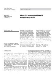
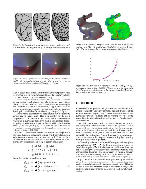
Figure 8: The boundary is subdivided only in every other step such<br />
th<strong>at</strong> a uniform 1-to-9 refinement of the triangular faces is achieved.<br />
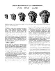
Figure 10: A decim<strong>at</strong>ed Stanford bunny was used as a <strong>subdivision</strong><br />
control mesh M 0 . We applied the ¢ 3-<strong>subdivision</strong> scheme 4 times<br />
(left). The right image shows the mean curv<strong>at</strong>ure distribution.<br />
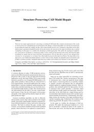
Figure 9: The use of univari<strong>at</strong>e smoothing rules <strong>at</strong> the boundaries<br />
enables the gener<strong>at</strong>ion of sharp fe<strong>at</strong>ure lines where two separ<strong>at</strong>e<br />
control meshes share an identical boundary polygon.<br />
interior edges. Edge flipping <strong>at</strong> the boundaries is not possible since<br />
the opposite triangle-m<strong>at</strong>e is missing. Hence, the boundary polygon<br />
is not modified in the first ¢ 3-<strong>subdivision</strong> step.<br />
As we already discussed in Section 2, the applic<strong>at</strong>ion of a second<br />
¢ 3-step has the overall effect of a tri-adic split where each original<br />
triangle is replaced by 9 new ones. Consequently, we have to apply<br />
a univari<strong>at</strong>e tri-section rule to the boundary polygon and connect the<br />
new vertices to the corresponding interior ones such th<strong>at</strong> a uniform<br />
1-to-9 split is established for each boundary triangle (cf. Fig. 8).<br />
The smoothing rules <strong>at</strong> the boundaries should only use boundary<br />
vertices and no interior ones. This is the simplest way to enable<br />
the gener<strong>at</strong>ion of C 0 creases in the interior of the surface (fe<strong>at</strong>ure<br />
lines) since it guarantees th<strong>at</strong> control meshes with identical boundary<br />
polygons will result in smooth surfaces with identical boundary<br />
curves [HDD+94] (cf. Fig. 9). More sophistic<strong>at</strong>ed techniques for<br />
the design of optimal boundary smoothing rules with normal control<br />
can be found in [BLZ99].<br />
For our ¢ 3-<strong>subdivision</strong> scheme we choose, for simplicity, a<br />
univari<strong>at</strong>e boundary <strong>subdivision</strong> scheme which reproduces cubic<br />
splines (maximum smoothness, minimum stencil). From the trivial<br />
tri-section mask for linear splines we can easily obtain the corresponding<br />
tri-section mask for cubic splines by convolution<br />
1<br />
31¤ 2¤ 3¤ 2¤ 1 £<br />
1<br />
31¤ 1¤ 1 ¥<br />
2<br />
1<br />
91¤ 3¤ 6¤ 7¤ 6¤ 3¤ 1<br />
1<br />
1<br />
31¤ 1¤ 1<br />
4¤ 10¤ 16¤ 19¤ 16¤ 10¤ 4¤ 271¤<br />
Hence the resulting smoothing rules are<br />
1<br />
p ¡ 3i¥1 1<br />
27<br />
£ 10p i¥1¢<br />
p ¡ 3i<br />
1<br />
27<br />
£ 4p i¥1¢<br />
p ¡ 3i 1<br />
1<br />
27<br />
£ p i¥1¢<br />
i¢<br />
16p p<br />
i¢<br />
i¢<br />
i 1¥<br />
i 1¥<br />
i 1¥ §<br />
(9)<br />
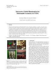
Figure 11: This plot shows the triangle count (Y : in ) K¤<br />
vs. approxim<strong>at</strong>ion<br />
error (X : in¦ log£ ε¥ ). The red curve is the complexity<br />
of the Loop-meshes, the blue curve the complexity of the ¢ 3-meshes.<br />
The r<strong>at</strong>io lies between 5% and 25%.<br />
6 Examples<br />
To demonstr<strong>at</strong>e the quality of the ¢ 3-<strong>subdivision</strong> surfaces we show<br />
a mesh gener<strong>at</strong>ed by uniformly refining a decim<strong>at</strong>ed version of the<br />
Stanford bunny (cf. Fig 10). The C 2 smoothness of the limit surface<br />
guarantees curv<strong>at</strong>ure continuity and the relaxing properties of the<br />
smoothing rules with only positive weights lead to a fair distribution<br />
of the curv<strong>at</strong>ure.<br />
We made several numerical experiments to check the rel<strong>at</strong>ive<br />
complexity of the adaptively refined meshes M k gener<strong>at</strong>ed either<br />
by ¢ 3-<strong>subdivision</strong> or by Loop-<strong>subdivision</strong>. For the stopping criterion<br />
in the adaptive refinement we used the local approxim<strong>at</strong>ion<br />
error of the current mesh (with all vertices projected onto the limit<br />
surface) to the limit surface. A reliable estim<strong>at</strong>ion of the exact approxim<strong>at</strong>ion<br />
error can be computed by constructing tight bounding<br />
envelopes as described in [KDS98].<br />
After testing various models with different geometric complexities<br />
over the range10¥2 ¤ 10¥7for the approxim<strong>at</strong>ion tolerance, we<br />
found th<strong>at</strong> adaptive ¢ 3-<strong>subdivision</strong> meshes usually need fewer triangles<br />
than adaptive Loop-<strong>subdivision</strong> surfaces to obtain the same<br />
approxim<strong>at</strong>ion tolerance. The improvement is typically between<br />
5% and 25% with an average <strong>at</strong> 10%. Fig. 11 shows the typical<br />
rel<strong>at</strong>ion between approxim<strong>at</strong>ion tolerance and mesh complexity.<br />
Fig. 12 shows another example mesh gener<strong>at</strong>ed by the adaptive<br />
¢ 3-<strong>subdivision</strong> scheme in comparison to the corresponding Loop<br />
<strong>subdivision</strong> surface defined by the same control mesh. This time<br />
we use a curv<strong>at</strong>ure dependent adaptive refinement str<strong>at</strong>egy: The<br />
<strong>subdivision</strong> level is determined by a discrete local curv<strong>at</strong>ure estim<strong>at</strong>ion.<br />
19p<br />
4p<br />
16p<br />
10p