sqrt(3) subdivision - Computer Graphics Group at RWTH Aachen

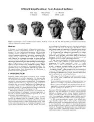
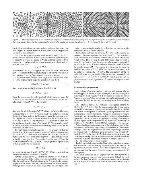
Figure 17: The local regularity of the subdivision surface at extraordinary vertices requires the injectivity of the characterisitc map. We show
the isoparameter lines for these maps in the vicinity of irregular vertices with valence n 3¤ 4¤ 5¤ 7, and 8 (form left to right).
involved factorizations and other polynomial transformations, we
now suggest a simpler approach where most of the computation
can be done automatically.
Let J n by the nth jet-operator restricted to V and J¥1
n its SVD
pseudo-inverse. Because J n has a non-trivial kernel (containing all
configurations where the points in V are uniformly sampled from
a degree 1 polynomial) its inverse cannot be well-defined. At
n¦
least we know that
J n J¥1
n J n J n
which means that if J¥1
n is applied to a set of nth order differences
J n V¥ it reconstructs the original data up to an error e which lies in
£
with J n e¥ 0. £
the kernel of J n , i.e., J¥1
If the subdivision scheme S has polynomial precision of order
1 this implies that S maps the kernel of J n into itself:
n¦
n £ J n £ V¥©¥ V¢ e
ker£ J S£ n ker£ J ¥¨¥ n § (11)
¥
As a consequence J n S£ e¥¨¥ 0 as well, and therefore
£
J n SJ¥1
n J n
J n S§
Since the operator on the right hand side of this equation maps the
vertices of the control mesh V k¡ to the nth differences on the next
refinement level J n £ V k 1¡ ¥ , the operator
S n : J n SJ¥1
n (12)
does map the nth differences J n £ V k¡ ¥ directly to the nth differences
on the next level J n £ V k 1¡ ¥ . This is exactly the difference scheme
that we have been looking for! In order to prove the convergence of
the subdivision scheme, we have to show that the maximum norm
of h n¥1 S n is below 1. Alternatively, it is sufficient to show that
the maximum singular value of the matrix h n¥1 S n is smaller than 1
since this provides a monotonically decreasing upper bound for the
maximum nth difference.
To verify the polynomial precision (11) for a given subdivision
matrix S we first generate another matrix K whose columns span
the kernel of J n . Notice that the dimension ker£ of J n is the dimension
of the space of bivariate degree 1 polynomials which
¥
n¦
is dimΠ 2 n¥1 1 2
£ n¢ 1¥ n. The matrix K can be read off from the
SVD decomposition of J n [GvL96]. The polynomial reproduction
is then guaranteed if the equation
SK K X (13)
has a matrix solution X £ K T K¥¥1 K T SK. If this is satisfied, we
find the nth difference scheme S n by (12).
For the analysis of our ¢ 3-subdivision scheme we let V be the
6-ring neighborhood of a vertex which consists of 127 vertices. Let
S be the single-step ¢ 3-subdivision matrix, R be the back-rotationby-permutation
matrix and D 10 the directional difference matrix.
Although these matrices are quite large, they are very sparse and
can be constructed quite easily (by a few lines of MatLab-code)
due to their block-circulant structure.
From these matrices we computeS RS 2 and a second directional
difference operator D 01 R 2 D R¥2 10 . The two directional
differences are combined to build the 3rd order jet-operator
J 3 (cf. (10)). Here we use the 3rd differences since we want to
prove C 2 continuity. From the singular value decomposition of J 3
we obtain the matrix K whose columns span the kernel of J 3 and
the pseudo-inverse J¥1
3 . The matrix K is then used to prove the
quadratic precision of S (cf. (13)) and the pseudo-inverse yields
the difference schemeS 3 J 3SJ¥1
3 . The contractivity of the 3rd
order difference scheme finally follows from the numerical estimation
S 2 3 J 3S 2 J¥1
3
0§ 78¨ 3¥4 which proves that the
¢ 3-subdivision scheme S generates C 2 surfaces for regular control
meshes.
Extraordinary vertices
In the vicinity of the extraordinary vertices with valence 6 we
have to apply a different analysis technique. After the convergence
in the regular mesh regions (which for subdivision meshes means
”almost everywhere”) has been shown, it is sufficient to analyse the
behavior of the limit surface at the remaining isolated extraordinary
points.
The intuition behind the sufficient convergence criteria by
[Rei95, Zor97, Pra98] is that the representation of the local neighborhood
V with respect to the eigenvector basis of the local subdivision
matrix S corresponds to a type of Taylor-expansion of the limit
surface at that extraordinary point. Hence, the eigenvectors (”eigenfunctions”)
have to satisfy some regularity criteria and the leading
eigenvalues have to guarantee an appropriate scaling of the tangential
and higher order components of the expansion. Especially the
conditions (5) have to be satisfied for all valences n 3¤¨§¨§©§¨¤ n max .
When checking the eigenstructure of the subdivision matrix S we
have to use a sufficiently large r-ring neighborhood V of the center
vertex p. In fact the neighborhood has to be large enough such that
the regular part of it defines a complete surface ring around p by
itself [Rei95]. In the case of ¢ 3-subdivision we hence have to use
r 4 rings around p (since 4 is the diameter of the subdivision basis
function’s support). This means we have to analyse a £ 10n¢ 1¥ ¨
£ 10n¢ 1¥ matrix where n is p’s valence.
Luckily the subdivision matrix S has a block circulant structure
and it turns out that the leading eigenvalues of S are exactly the
eigenvalues we found in (4). Since those eigenvalues satisfy (5)
we conclude that the matrix S has the appropriate structure for C 1
convergence.
The exact condition on the eigenvectors and the injectivity of
the corresponding characteristic map are quite difficult to check
strictly. We therefore restrict ourselves to the numerical verification
by sketching the iso-parameter lines of the characterisitc map in
Fig. 17.