CP/MM Tutorial
CP/MM Tutorial
CP/MM Tutorial

You also want an ePaper? Increase the reach of your titles
YUMPU automatically turns print PDFs into web optimized ePapers that Google loves.
<strong>CP</strong>/<strong>MM</strong> <strong>Tutorial</strong><br />
Jülich, 26/07/2012<br />
Emiliano Ippoliti: e.ippoliti@grs-sim.de<br />
Preliminary Information<br />
To reproduce the calculations in the tutorial and performed the exercises therein you<br />
need a workstation where to run the required programs that should be already<br />
installed. To this aim, we will use the main supercomputer of the Aachen<br />
Rechenzentrum. In order to access this HPC cluster, you need a user account. Each<br />
student who are already registered in the Aachen TIM-System can activate an account<br />
on their own through the following procedure:<br />
• Access your TIM webpage manager:<br />
https://tim.rz.rwth-aachen.de/enrole/logon<br />
by inserting your credentials.<br />
• Click on the “Manage Accounts” icon in the menu at the left of the page.<br />
• Press the “New” button on the main frame of the page to request the activation<br />
of a new service.<br />
• Tick the “Hochleistungsrechnen RWTH Aachen” entry and press “Continue”.<br />
• Tick the “Ich habe die Nutzungs-/Lizenzbedingungen gelesen und stimme zu”<br />
and press the “Submit” button.<br />
In some minutes/hours your account should be created.<br />
To enter the cluster you can use the ssh command from a terminal window in your<br />
laptop:<br />
ssh –Y @cluster.rz.rwth-aachen.de<br />
For data transfer from and to your laptop use the scp command.<br />
A very useful user guide for an exhaustive quick start with such a machine can be<br />
found at the address:<br />
http://www.rz.rwth-aachen.de/global/show_document.asp?id=aaaaaaaaaacfhzd<br />
It is strongly suggested to read it and referes to that in case of problem with running<br />
jobs.<br />
Introduction<br />
We want to study the effect of the solvent (water) and the temperature on the dipole<br />
moment of an acetone molecule. To accomplish that we will resort to several different
software (MOLDEN, <strong>CP</strong>MD, VMD, Gaussian09, Amber, GROMOS, etc) in order to<br />
let you taste the everyday working in the biophysical field.<br />
The procedure can be summarized in the following steps:<br />
1. Calculate the dipole moment D v of acetone in vacuum<br />
2. Perform a QM/<strong>MM</strong> molecular dynamics simulation for the acetone in a<br />
classical water box at room temperature.<br />
3. Calculate the dipole moment D for some random snapshots of this simulation<br />
and take the mean value<br />
4. Calculate the difference D - D v<br />
Each file mentioned in this tutorial (in bold) can be found on the Aachen<br />
supercomputer in the folder:<br />
/home/ei250498/<strong>Tutorial</strong>s/ACETONE<br />
under the subfolder whose name starts with the number of the corresponding section<br />
of this tutorial.<br />
To do your tests and exercises, work in your own folder in $WORK filesystem by<br />
creating a folder there by the command:<br />
Then to go to your folder:<br />
mkdir $WORK/Q<strong>MM</strong>M_<strong>Tutorial</strong><br />
cd $WORK/Q<strong>MM</strong>M_<strong>Tutorial</strong><br />
1 - Where to start?<br />
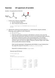
Acetone is the organic compound with the formula (CH3) 2 CO. This colorless, mobile,<br />
flammable liquid is the simplest example of the ketones:<br />
Figure 1. Acetone<br />
To obtain an initial structure we use the MOLDEN program. 1 As for all the programs<br />
mentioned in this tutorial, the first time in each session you want to use molden you<br />
need to initialize the environment in order to be able to recall it. This can be done<br />
with a “source” command:<br />
source /home/ei250498/PROGRAMS/MODULES/molden.sh<br />
1 http://www.cmbi.ru.nl/molden/molden.html <br />
2 An online general guide for the ZMAT Editor can be found at the web address:
Then, you can run molden by simply typing:<br />
molden &<br />
In the Molden Control panel at the right, deselect the “Shade” button and press on the<br />
“ZMAT Editor” button that is a tool to create and/or manipulate structures on screen<br />
and to optimize the structures on a force field level.<br />
The use of the editor is rather intuitive. 2 In the following a synthetic list of the steps to<br />
create the acetone molecule:<br />
• Press “Add line”<br />
• Select Carbon from the Periodic Table<br />
• Press “Substitute atom by Fragment” and without releasing the mouse button<br />
select the –HC=O<br />
• Press “Add line”<br />
• Select Hydrogen from the Periodic Table<br />
• Click, in the Main screen, on the 4 atoms H,C,O,H in sequence to define the<br />
connectivity of the new H atom in the molecule<br />
• Highlight a Hydrogen by pressing on the atom in the Main screen or in the list<br />
of atoms in Zmat Editor<br />
• Press “Substitute atom by Fragment” and without releasing the mouse button<br />
select the –CH3<br />
• Do the same for the other Hydrogen<br />
Then, we can save the structure in the xyz format by writing the name of the file in<br />
the field “File name?”, choosing the “XYZ” format in the menu which appear when<br />
you press on the square “Cartesian” at the right bottom and finally pressing “Write Z-<br />
Matrix”.<br />
Close the ZMAT Editor by clicking the “Close” button on the right top and then by<br />
pressing on the button with a skull.<br />
2 - Dipole moment in vacuum<br />
We will use <strong>CP</strong>MD to calculate the dipole moment of acetone in gas phase.<br />
To initialize the environment and be able to use <strong>CP</strong>MD:<br />
source /home/ei250498/PROGRAMS/MODULES/cpmd.sh<br />
Any program can be run interactively on the login node. In the following we report<br />
the command to do that. However, if your job is supposed to run for more than 5<br />
minutes this is NOT a good practice: longer jobs should be run on the computational<br />
node by using the batch system. This can be accomplished by writing a simple batch<br />
script where you insert the information about your job and then submit the request to<br />
the batch system through the command:<br />
2 An online general guide for the ZMAT Editor can be found at the web address: <br />
http://www.cmbi.ru.nl/molden/zmat/zmat.html#add
sub < <br />
Some batch script templates called launch_XXX.job can be found in:<br />
/home/ei250498/TUTORIALS/ACETONE<br />
If you open them you will found some initial lines starting with #BSUB word that<br />
represents commands for the batch system:<br />
#BSUB -J Template<br />
#BSUB -o output<br />
#BSUB -e error<br />
#BSUB -n 2<br />
#BSUB -W 00:15<br />
#BSUB -M 700<br />
#BSUB -a intelmpi<br />
ß Batch system’s job name<br />
ß Filename of the batch system’s output messages (and error if no option -e used)<br />
ß Filename of the batch system’s error messages<br />
ß Number of cores to be reserve for the job<br />
ß Hard runtime limit: after the expiration of this time (here 15’) the job will be killed<br />
ß Set the per-process memory limit in MB<br />
ß Specify which MPI version you want to use in the parallel run<br />
followed by some lines which are the commands that the batch system has to run on<br />
the computational nodes and that are similar to the ones you use in the interactive<br />
way.<br />
Refer to the HPC user guide for a more detailed description of all the useful<br />
commands available for the batch script.<br />
To check the status of your batched jobs you can use the command:<br />
bjobs –w<br />
and to remove a job from the batch list you can use the command:<br />
bkill <br />
where the job_id can be read from the list got with the bjobs command.<br />
A batch script template called launch.job can be found in:<br />
/home/ei250498/TUTORIALS/ACETONE<br />
Refer to the HPC user guide to learn how to create a batch script for your jobs.<br />
To run <strong>CP</strong>MD with for example 2 cores (everything on the same line):<br />
mpirun –np 2 cpmd.x /home/ei250498/PROGRAMS/SRC/cpmd/PP<br />
> &<br />
/home/ei250498/PROGRAMS/SRC/cpmd/PP is the location where <strong>CP</strong>MD will look for<br />
the pseudopotentials files which will be specified in the input file. All the<br />
pseudopotentials we will use are already present there.<br />
In order to calculate the dipole moment of the acetone in vacuum we first have to<br />
optimize the geometry of the molecule we have constructed in the previous step. So,
we need to write an appropriate input file according the syntax of <strong>CP</strong>MD. 3 By your<br />
favorite editor, write down the opt_geo.inp text file:<br />
&INFO<br />
Acetone molecule<br />
Geometry optimization<br />
&END<br />
&<strong>CP</strong>MD<br />
OPTIMIZE GEOMETRY XYZ<br />
CONVERGENCE ORBITALS<br />
1.0d-7<br />
CONVERGENCE GEOMETRY<br />
7.0d-4<br />
&END<br />
&SYSTEM<br />
ANGSTROM<br />
SY<strong>MM</strong>ETRY<br />
ORTHORHOMBIC<br />
CELL ABSOLUTE<br />
10.6 10.0 9.8 0.0 0.0 0.0<br />
CUTOFF<br />
70.<br />
&END<br />
&DFT<br />
FUNCTIONAL BLYP<br />
&END<br />
&ATOMS<br />
*C_MT_BLYP.psp KLEINMAN-BYLANDER<br />
LMAX=D<br />
3<br />
0.000000 0.000000 0.000000<br />
1.367073 0.000000 -0.483333<br />
-0.683537 -1.183920 -0.483333<br />
*O_MT_BLYP.psp KLEINMAN-BYLANDER<br />
LMAX=D<br />
1<br />
0.000000 0.000000 1.220000<br />
*H_MT_BLYP.psp KLEINMAN-BYLANDER<br />
LMAX=P<br />
6<br />
1.367073 0.000000 -1.572333<br />
1.880433 0.889165 -0.120333<br />
1.880433 -0.889165 -0.120333<br />
-0.683537 -1.183920 -1.572333<br />
-0.170177 -2.073085 -0.120333<br />
-1.710256 -1.183920 -0.120333<br />
&END<br />
<strong>CP</strong>MD Input file<br />
3 <strong>CP</strong>MD manual: http://www.cpmd.org/manual.pdf
Any <strong>CP</strong>MD input file is organized in sections that start with &NAME and end with<br />
&END. Everything outside those sections is ignored. Also all keywords have to be in<br />
upper case or else they will be ignored. The sequence of the sections does not matter,<br />
nor does the order of keywords (except in some special case reported in the manual).<br />
A minimal input file must have a &<strong>CP</strong>MD, &SYSTEM, and an &ATOMS section.<br />
This input file starts with an (optional) &INFO section. This section allows you to put<br />
comments about the calculation into the input file and they will be repeated in the<br />
output file. This can be very useful to identify and match your input and output files.<br />
The first part of &<strong>CP</strong>MD section instructs the program to do a geometry optimization<br />
(XYZ suboption specify you want the final structure also in xyz format in a file called<br />
GEOMETRY.xyz and a ’trajectory’ of the optimization in a file named GEO_OPT.xyz)<br />
with a tight wavefunction and geometry convergence criterions respectively (default<br />
10 -5 and 5*10 -4 ).<br />
The &SYSTEM section contains various parameters related to the simulation cell and<br />
the representation of the electronic structure. The keywords SY<strong>MM</strong>ETRY, CELL and<br />
CUTOFF are required and define the (periodic) symmetry, shape, and size of the<br />
simulation cell, as well as the plane wave energy cutoff (i.e. the size of the basis set),<br />
respectively. The keyword ANGSTROM specify that the atomic coordinates and the<br />
supercell parameters and several other parameters are read in Ångströms (pay<br />
attention: default is atomic units (a.u.) which are always used internally). We define a<br />
primitive orthorhombic cell with the lattice constants obtained by adding 7 Å in each<br />
direction to the dimension of the system: the cell has to be large enough to avoid<br />
significant interactions of the acetone molecule and its electron structure with its<br />
periodic neighbors. In <strong>CP</strong>MD all calculations are periodic. Do always a convergence<br />
test looking for example at the total energy value when you increase the box size!<br />
The &DFT section is used to select the density functional (FUNCTIONAL) and<br />
related parameters. In this case we use the gradient corrected BLYP functional 4 (local<br />
density approximation is the default).<br />
Finally, the &ATOMS section is needed to specify the atom coordinates and the<br />
pseudopotential(s), that are used to represent them. The coordinates are taken from<br />
the structure written by MOLDEN.<br />
The input for a new atom type is started with a ``*'' in the first column. This line<br />
further contains the file name where to find the pseudopotential information starting<br />
in column 2 and several labels as KLEINMAN-BYLANDER, in our case, which specifies<br />
the method to be used for the calculation of the nonlocal parts of the pseudopotential<br />
(this method is extremely efficient but also accurate).<br />
The next line contains information on the nonlocality of the pseudopotential: you can<br />
specify the maximum l-quantum number with ``LMAX= l '' where l is S, P or D. 5<br />
On the following lines the coordinates for this atomic species have to be given.<br />
4 A.D. Becke, J.Chem.Phys. 98 (1993) 5648-‐5652; C. Lee, W. Yang, R.G. Parr, Phys. Rev. B 37 <br />
(1988) 785-‐789. <br />
5 If this is the only input, the program assumes that LMAX is the l for the local<br />
potential. You can use another local function by specifying ``LOC= ''. In addition it is<br />
possible to assign the local potential to a further potential with ``SKIP= ''.
The first line gives the number of atoms of the current type.<br />
---<br />
If you start the geometry optimization:<br />
mpirun -np 2 cpmd.x opt_geo.inp /home/ei250498/PROGRAMS/SRC/cpmd/PP ><br />
opt_geo.out &<br />
the calculation should be completed in less than a minute 5 minutes (use<br />
tail –f opt_geo.out<br />
to monitor the different steps of the calculation reported in the output file).<br />
<strong>CP</strong>MD Output file<br />
Look at the output file to understand all the information which we can find there.<br />
At the beginning there is the header where one can see, when the run was started,<br />
what version of <strong>CP</strong>MD was used, and when it was compiled:<br />
PROGRAM <strong>CP</strong>MD STARTED AT: Tue Jun 1 19:32:59 2010<br />
SETCNST| USING: CODATA 2006 UNITS<br />
****** ****** **** **** ******<br />
******* ******* ********** *******<br />
*** ** *** ** **** ** ** ***<br />
** ** *** ** ** ** ** **<br />
** ******* ** ** ** **<br />
*** ****** ** ** ** ***<br />
******* ** ** ** *******<br />
****** ** ** ** ******<br />
VERSION 3.13.2<br />
COMPILED WITH GROMOS-AMBER QM/<strong>MM</strong> SUPPORT<br />
COPYRIGHT<br />
IBM RESEARCH DIVISION<br />
MPI FESTKOERPERFORSCHUNG STUTTGART<br />
The <strong>CP</strong>MD consortium<br />
Home Page: http://www.cpmd.org<br />
Mailing List: cpmd-list@cpmd.org<br />
E-mail: cpmd@cpmd.org<br />
*** Jan 10 2011 -- 16:03:39 ***<br />
Then, we find some technical information about the environment (machine, user,<br />
directory, input file, process id) where this job was run:<br />
THE INPUT FILE IS:<br />
opt_geo.inp<br />
THIS JOB RUNS ON:<br />
cluster-linux.rz.RWTH-Aachen.DE<br />
THE CURRENT DIRECTORY IS:<br />
/home/ei250498/<strong>Tutorial</strong>s/ACETONE/2-<strong>CP</strong>MD<br />
THE TEMPORARY DIRECTORY IS:<br />
/home/ei250498/<strong>Tutorial</strong>s/ACETONE/2-<strong>CP</strong>MD<br />
THE PROCESS ID IS: 28735<br />
Next are the contents of the &INFO section copied to the output:
******************************************************************************<br />
* INFO - INFO - INFO - INFO - INFO - INFO - INFO - INFO - INFO - INFO - INFO *<br />
******************************************************************************<br />
* Acetone molecule *<br />
* Geometry optimization *<br />
******************************************************************************<br />
Next section contain a summary of some of the parameters read in from the &<strong>CP</strong>MD<br />
section, or their respective default settings; for example the convergence threshold for<br />
wavefunction optimization (set manually) or the maximum number of iterations<br />
(default):<br />
OPTIMIZATION OF IONIC POSITIONS<br />
PATH TO THE RESTART FILES: ./<br />
GRAM-SCHMIDT ORTHOGONALIZATION<br />
MAXIMUM NUMBER OF STEPS:<br />
10000 STEPS<br />
MAXIMUM NUMBER OF ITERATIONS FOR SC:<br />
10000 STEPS<br />
PRINT INTERMEDIATE RESULTS EVERY<br />
10001 STEPS<br />
STORE INTERMEDIATE RESULTS EVERY<br />
10001 STEPS<br />
STORE INTERMEDIATE RESULTS EVERY 10001 SELF-CONSISTENT STEPS<br />
NUMBER OF DISTINCT RESTART FILES: 1<br />
TEMPERATURE IS CALCULATED ASSUMING EXTENDED BULK BEHAVIOR<br />
FICTITIOUS ELECTRON MASS: 400.0000<br />
TIME STEP FOR ELECTRONS: 5.0000<br />
TIME STEP FOR IONS: 5.0000<br />
CONVERGENCE CRITERIA FOR WAVEFUNCTION OPTIMIZATION: 1.0000E-06<br />
WAVEFUNCTION OPTIMIZATION BY PRECONDITIONED DIIS<br />
THRESHOLD FOR THE WF-HESSIAN IS 0.5000<br />
MAXIMUM NUMBER OF VECTORS RETAINED FOR DIIS: 10<br />
STEPS UNTIL DIIS RESET ON POOR PROGRESS: 10<br />
FULL ELECTRONIC GRADIENT IS USED<br />
CONVERGENCE CRITERIA FOR GEOMETRY OPTIMIZATION: 3.000000E-04<br />
GEOMETRY OPTIMIZATION BY GDIIS/BFGS<br />
SIZE OF GDIIS MATRIX: 5<br />
GEOMETRY OPTIMIZATION IS SAVED ON FILE GEO_OPT.xyz<br />
EMPIRICAL INITIAL HESSIAN (DISCO PARAMETRISATION)<br />
SPLINE INTERPOLATION IN G-SPACE FOR PSEUDOPOTENTIAL FUNCTIONS<br />
NUMBER OF SPLINE POINTS: 5000<br />
The exchange correlation functionals are reported in the lines coming immediately<br />
after:<br />
EXCHANGE CORRELATION FUNCTIONALS<br />
LDA EXCHANGE: SLATER (ALPHA = 0.66667)<br />
LDA CORRELATION:<br />
LEE, YANG & PARR<br />
[C.L. LEE, W. YANG, AND R.G. PARR, PRB 37 785 (1988)]<br />
GRADIENT CORRECTED FUNCTIONAL<br />
DENSITY THRESHOLD:<br />
1.00000E-08<br />
EXCHANGE ENERGY<br />
[A.D. BECKE, PHYS. REV. A 38, 3098 (1988)]<br />
PARAMETER BETA: 0.004200<br />
CORRELATION ENERGY<br />
[LYP: C.L. LEE ET AL. PHYS. REV. B 37, 785 (1988)]<br />
At this point of the output you find which and how many atoms (and their coordinates<br />
in a.u.), electrons and states (we are doing a closed shell calculation, so there are only<br />
doubly occupied states) are in the system, and what pseudopotentials were used with<br />
which settings:<br />
*** DETSP| SIZE OF THE PROGRAM IS 3700/ 119392 kBYTES ***<br />
***************************** ATOMS ****************************
NR TYPE X(bohr) Y(bohr) Z(bohr) MBL<br />
1 C 0.000000 0.000000 0.000000 3<br />
2 C 2.583394 0.000000 -0.913367 3<br />
3 C -1.291698 -2.237285 -0.913367 3<br />
4 O 0.000000 0.000000 2.305466 3<br />
5 H 2.583394 0.000000 -2.971279 3<br />
6 H 3.553503 1.680278 -0.227396 3<br />
7 H 3.553503 -1.680278 -0.227396 3<br />
8 H -1.291698 -2.237285 -2.971279 3<br />
9 H -0.321588 -3.917563 -0.227396 3<br />
10 H -3.231915 -2.237285 -0.227396 3<br />
****************************************************************<br />
NUMBER OF STATES: 12<br />
NUMBER OF ELECTRONS: 24.00000<br />
CHARGE: 0.00000<br />
ELECTRON TEMPERATURE(KELVIN): 0.00000<br />
OCCUPATION<br />
2.0 2.0 2.0 2.0 2.0 2.0 2.0 2.0 2.0 2.0 2.0 2.0<br />
============================================================<br />
| Pseudopotential Report Tue Jan 14 09:55:25 1997 |<br />
------------------------------------------------------------<br />
| Atomic Symbol : C |<br />
| Atomic Number : 6 |<br />
| Number of core states : 1 |<br />
| Number of valence states : 2 |<br />
| Exchange-Correlation Functional : |<br />
| Slater exchange : .6667 |<br />
| LDA correlation : Lee-Yang-Parr |<br />
| Exchange GC : Becke (1988) |<br />
| Correlation GC : Lee-Yang-Parr |<br />
| Electron Configuration : N L Occupation |<br />
| 1 S 2.0000 |<br />
| 2 S 2.0000 |<br />
| 2 P 2.0000 |<br />
| Full Potential Total Energy -37.702121 |<br />
| Trouiller-Martins normconserving PP |<br />
| n l rc energy |<br />
| 2 S 1.2300 -.49630 |<br />
| 2 P 1.2300 -.19186 |<br />
| 3 D .7159 -.19186 |<br />
| Number of Mesh Points : 615 |<br />
| Pseudoatom Total Energy -5.370516 |<br />
============================================================<br />
============================================================<br />
| Pseudopotential Report Thu Nov 30 13:19:26 1995 |<br />
------------------------------------------------------------<br />
| Atomic Symbol : O |<br />
| Atomic Number : 8 |<br />
| Number of core states : 1 |<br />
| Number of valence states : 2 |<br />
| Exchange-Correlation Functional : |<br />
| Slater exchange : .6667 |<br />
| LDA correlation : Lee-Yang-Parr |<br />
| Exchange GC : Becke (1988) |<br />
| Correlation GC : Lee-Yang-Parr |<br />
| Electron Configuration : N L Occupation |<br />
| 1 S 2.0000 |<br />
| 2 S 2.0000 |<br />
| 2 P 4.0000 |<br />
| Full Potential Total Energy -75.023693 |<br />
| Trouiller-Martins normconserving PP |<br />
| n l rc energy |<br />
| 2 S 1.0500 -.87404 |<br />
| 2 P 1.0500 -.33186 |<br />
| 3 D 1.0500 -.33186 |<br />
| Number of Mesh Points : 631 |<br />
| Pseudoatom Total Energy -15.775323 |<br />
============================================================<br />
============================================================<br />
| Pseudopotential Report Thu Nov 30 13:17:19 1995 |<br />
------------------------------------------------------------<br />
| Atomic Symbol : H |<br />
| Atomic Number : 1 |<br />
| Number of core states : 0 |<br />
| Number of valence states : 1 |
| Exchange-Correlation Functional : |<br />
| Slater exchange : .6667 |<br />
| LDA correlation : Lee-Yang-Parr |<br />
| Exchange GC : Becke (1988) |<br />
| Correlation GC : Lee-Yang-Parr |<br />
| Electron Configuration : N L Occupation |<br />
| 1 S 1.0000 |<br />
| Full Potential Total Energy -.462611 |<br />
| Trouiller-Martins normconserving PP |<br />
| n l rc energy |<br />
| 1 S .5000 -.24002 |<br />
| 2 P .5000 -.24002 |<br />
| Number of Mesh Points : 511 |<br />
| Pseudoatom Total Energy -.462591 |<br />
============================================================<br />
****************************************************************<br />
* ATOM MASS RAGGIO NLCC PSEUDOPOTENTIAL *<br />
* C 12.0112 1.2000 NO KLEINMAN S NONLOCAL *<br />
* P NONLOCAL *<br />
* D LOCAL *<br />
* O 15.9994 1.2000 NO KLEINMAN S NONLOCAL *<br />
* P NONLOCAL *<br />
* D LOCAL *<br />
* H 1.0080 1.2000 NO KLEINMAN S NONLOCAL *<br />
* P LOCAL *<br />
****************************************************************<br />
Then, a section about how the calculation is distributed through the cores: here you<br />
can understand if something wrong happened and you run for example only a serial<br />
job! Here below an example of this section by using 8 cores:<br />
PARAPARAPARAPARAPARAPARAPARAPARAPARAPARAPARAPARAPARAPARAPARAPARA<br />
N<strong>CP</strong>U NGW NHG PLANES GXRAYS HXRAYS ORBITALS Z-PLANES<br />
0 4333 34682 13 246 976 1 1<br />
1 4335 34684 14 246 976 2 1<br />
2 4336 34639 13 243 975 1 1<br />
3 4336 34676 14 244 976 2 1<br />
4 4334 34682 13 244 976 1 1<br />
5 4332 34670 14 244 976 2 1<br />
6 4338 34676 13 244 976 1 1<br />
7 4342 34680 14 244 976 2 1<br />
G=0 COMPONENT ON PROCESSOR : 2<br />
PARAPARAPARAPARAPARAPARAPARAPARAPARAPARAPARAPARAPARAPARAPARAPARA<br />
*** LOADPA| SIZE OF THE PROGRAM IS 10260/ 120760 kBYTES ***<br />
OPENMPOPENMPOPENMPOPENMPOPENMPOPENMPOPENMPOPENMPOPENMPOPENMPOPEN<br />
NUMBER OF <strong>CP</strong>US PER TASK 1<br />
OPENMPOPENMPOPENMPOPENMPOPENMPOPENMPOPENMPOPENMPOPENMPOPENMPOPEN<br />
*** RGGEN| SIZE OF THE PROGRAM IS 11492/ 121976 kBYTES ***<br />
The following part of the output we see a summary of the settings read in from the<br />
&SYSTEM section of the input file or their corresponding defaults and some derived<br />
parameters (density cutoff, number of plane waves):<br />
************************** SUPERCELL ***************************<br />
SY<strong>MM</strong>ETRY:<br />
ORTHORHOMBIC<br />
LATTICE CONSTANT(a.u.): 20.03110<br />
CELL DIMENSION: 20.0311 0.9434 0.9245 0.0000 0.0000 0.0000<br />
VOLUME(OMEGA IN BOHR^3): 7010.16987<br />
LATTICE VECTOR A1(BOHR): 20.0311 0.0000 0.0000<br />
LATTICE VECTOR A2(BOHR): 0.0000 18.8973 0.0000<br />
LATTICE VECTOR A3(BOHR): 0.0000 0.0000 18.5193<br />
RECIP. LAT. VEC. B1(2Pi/BOHR): 0.0499 0.0000 0.0000<br />
RECIP. LAT. VEC. B2(2Pi/BOHR): 0.0000 0.0529 0.0000<br />
RECIP. LAT. VEC. B3(2Pi/BOHR): 0.0000 0.0000 0.0540<br />
REAL SPACE MESH: 108 108 100<br />
WAVEFUNCTION CUTOFF(RYDBERG): 70.00000<br />
DENSITY CUTOFF(RYDBERG): (DUAL= 4.00) 280.00000
NUMBER OF PLANE WAVES FOR WAVEFUNCTION CUTOFF: 34686<br />
NUMBER OF PLANE WAVES FOR DENSITY CUTOFF: 277389<br />
****************************************************************<br />
Here we see how <strong>CP</strong>MD generates the initial guess for the wavefunction<br />
optimization. In this case it uses a superposition of atomic wavefunctions using an<br />
(internal) minimal Slater basis:<br />
*** RINFORCE| SIZE OF THE PROGRAM IS 16052/ 127264 kBYTES ***<br />
*** FFTPRP| SIZE OF THE PROGRAM IS 19764/ 128656 kBYTES ***<br />
GENERATE ATOMIC BASIS SET<br />
C SLATER ORBITALS<br />
2S ALPHA= 1.6083 OCCUPATION= 2.00<br />
2P ALPHA= 1.5679 OCCUPATION= 2.00<br />
O SLATER ORBITALS<br />
2S ALPHA= 2.2458 OCCUPATION= 2.00<br />
2P ALPHA= 2.2266 OCCUPATION= 4.00<br />
H SLATER ORBITALS<br />
1S ALPHA= 1.0000 OCCUPATION= 1.00<br />
INITIALIZATION TIME:<br />
0.39 SECONDS<br />
*** GMOPTS| SIZE OF THE PROGRAM IS 24656/ 141780 kBYTES ***<br />
*** PHFAC| SIZE OF THE PROGRAM IS 24764/ 152468 kBYTES ***<br />
*** ATOMWF| SIZE OF THE PROGRAM IS 25784/ 154300 kBYTES ***<br />
ATRHO| CHARGE(R-SPACE): 24.000000 (G-SPACE): 24.000000<br />
****************************************************************<br />
* ATOMIC COORDINATES *<br />
****************************************************************<br />
1 C 0.000000 0.000000 0.000000<br />
2 C 2.583394 0.000000 -0.913367<br />
3 C -1.291698 -2.237285 -0.913367<br />
4 O 0.000000 0.000000 2.305466<br />
5 H 2.583394 0.000000 -2.971279<br />
6 H 3.553503 1.680278 -0.227396<br />
7 H 3.553503 -1.680278 -0.227396<br />
8 H -1.291698 -2.237285 -2.971279<br />
9 H -0.321588 -3.917563 -0.227396<br />
10 H -3.231915 -2.237285 -0.227396<br />
****************************************************************<br />
From the following statement in the output you can see that the Hessian has been<br />
initialized from a simple guess assuming a molecule with some specified bonds. This<br />
behavior can be controlled with the keyword HESSIAN. For bulk systems or<br />
complicated molecules, it may be better to start from a unit Hessian instead:<br />
INITIALIZE EMPIRICAL HESSIAN<br />
><br />
2 1 3 1 4 1 5 2 6 2<br />
7 2 8 3 9 3 10 3<br />
><br />
5 1 5 3 6 1 6 4 7 1<br />
7 3 7 4 8 1 8 2 9 1<br />
9 2 9 4 10 1 10 4<br />
TOTAL NUMBER OF MOLECULAR STRUCTURES: 1<br />
****************************************************************<br />
* ATOMIC COORDINATES *<br />
****************************************************************<br />
1 C 0.000000 0.000000 0.000000<br />
2 C 2.583394 0.000000 -0.913367<br />
3 C -1.291698 -2.237285 -0.913367<br />
4 O 0.000000 0.000000 2.305466<br />
5 H 2.583394 0.000000 -2.971279<br />
6 H 3.553503 1.680278 -0.227396<br />
7 H 3.553503 -1.680278 -0.227396<br />
8 H -1.291698 -2.237285 -2.971279<br />
9 H -0.321588 -3.917563 -0.227396<br />
10 H -3.231915 -2.237285 -0.227396
****************************************************************<br />
Now the program is ready to start the geometry optimization. You can follow the<br />
progress of the optimization in the output file:<br />
<strong>CP</strong>U TIME FOR INITIALIZATION<br />
0.81 SECONDS<br />
================================================================<br />
= GEOMETRY OPTIMIZATION =<br />
================================================================<br />
NFI GEMAX CNORM ETOT DETOT T<strong>CP</strong>U<br />
EWALD| SUM IN REAL SPACE OVER<br />
1* 1* 1 CELLS<br />
1 3.015E-02 4.345E-03 -35.648938 -3.565E+01 0.51<br />
2 1.889E-02 1.442E-03 -36.307687 -6.587E-01 0.46<br />
3 1.904E-02 7.725E-04 -36.379166 -7.148E-02 0.46<br />
…<br />
26 1.294E-06 1.055E-07 -36.415776 -2.343E-09 0.48<br />
27 9.933E-07 7.580E-08 -36.415776 -1.233E-09 0.48<br />
RESTART INFORMATION WRITTEN ON FILE<br />
./RESTART.1<br />
ATOM COORDINATES GRADIENTS (-FORCES)<br />
1 C 0.0000 0.0000 0.0000 -4.443E-02 7.697E-02 -5.004E-02<br />
2 C 2.5834 0.0000 -0.9134 -3.769E-02 -4.835E-02 4.876E-02<br />
3 C -1.2917 -2.2373 -0.9134 6.088E-02 8.661E-03 4.903E-02<br />
4 O 0.0000 0.0000 2.3055 3.158E-02 -5.469E-02 -6.270E-02<br />
5 H 2.5834 0.0000 -2.9713 -1.090E-02 -5.915E-05 8.858E-03<br />
6 H 3.5535 1.6803 -0.2274 -9.255E-03 -3.027E-03 -2.712E-04<br />
7 H 3.5535 -1.6803 -0.2274 6.917E-04 3.287E-03 -1.830E-03<br />
8 H -1.2917 -2.2373 -2.9713 5.515E-03 9.402E-03 8.862E-03<br />
9 H -0.3216 -3.9176 -0.2274 -3.189E-03 1.061E-03 -1.824E-03<br />
10 H -3.2319 -2.2373 -0.2274 7.229E-03 6.496E-03 -2.472E-04<br />
FILE GEO_OPT.xyz EXISTS, NEW DATA WILL BE APPENDED<br />
****************************************************************<br />
*** TOTAL STEP NR. 27 GEOMETRY STEP NR. 1 ***<br />
*** GNMAX= 7.696852E-02 ETOT= -36.415776 ***<br />
*** GNORM= 3.227866E-02 DETOT= 0.000E+00 ***<br />
*** CNSTR= 0.000000E+00 T<strong>CP</strong>U= 12.89 ***<br />
****************************************************************<br />
1 2.130E-02 5.311E-03 -35.580799 8.350E-01 0.46<br />
2 1.574E-02 1.566E-03 -36.324351 -7.436E-01 0.46<br />
3 5.503E-03 8.729E-04 -36.400043 -7.569E-02 0.46<br />
...<br />
A geometry optimization is not much else than repeated wavefunction optimizations,<br />
where the positions of the atoms are updated according to the forces acting on them.<br />
In the first part above you can see, the wavefunction optimization. The columns have<br />
the following meaning:<br />
• NFI step number (number of finite iterations)<br />
• GEMAX largest off-diagonal component<br />
• CNORM average of the off-diagonal components<br />
• ETOT total energy DETOT change in total energy<br />
• T<strong>CP</strong>U time used for this step<br />
One can see that the calculation stops after the convergence criterion of 1.0d-6 has<br />
been reached for the GEMAX value.<br />
After printing the positions and forces of the atoms you see a small report block and<br />
then another wavefunction optimization starts. The numbers for GNMAX, GNORM,<br />
and CNSTR stand for the largest absolute component of the force on any atom,
average force on the atoms, and the largest absolute component of a constraint force<br />
on the atoms respectively. They allow you to monitor the progress of the convergence<br />
of the geometry optimization.<br />
Finally, at the end of the geometry optimization, you can see that the forces and the<br />
total energy have decreased from their initial values as it is to be expected:<br />
****************************************************************<br />
*** TOTAL STEP NR. 3737 GEOMETRY STEP NR. 214 ***<br />
*** GNMAX= 2.827646E-04 [3.64E-02] ETOT= -36.489908 ***<br />
*** GNORM= 1.395703E-04 DETOT= -1.769E-05 ***<br />
*** CNSTR= 0.000000E+00 T<strong>CP</strong>U= 9.63 ***<br />
****************************************************************<br />
================================================================<br />
= END OF GEOMETRY OPTIMIZATION =<br />
================================================================<br />
and we have the final summary of the results; the atom coordinates and a breakdown<br />
of the total energy into the various components:<br />
RESTART INFORMATION WRITTEN ON FILE<br />
./RESTART.1<br />
****************************************************************<br />
* *<br />
* FINAL RESULTS *<br />
* *<br />
****************************************************************<br />
ATOM COORDINATES GRADIENTS (-FORCES)<br />
1 C 0.3033 -0.3710 0.4996 2.238E-04 -3.750E-05 -1.867E-04<br />
2 C 2.8157 0.1207 -0.8206 -2.828E-04 1.186E-04 1.534E-04<br />
3 C -1.4005 -2.3884 -0.6592 -1.866E-05 -5.129E-05 1.748E-04<br />
4 O -0.3055 0.7755 2.4178 1.488E-05 -9.553E-05 2.593E-04<br />
5 H 2.5171 0.5750 -2.8280 7.045E-06 -1.029E-04 -2.289E-04<br />
6 H 3.8187 1.6721 0.1124 -6.949E-05 1.507E-04 -3.226E-05<br />
7 H 3.9948 -1.5943 -0.7676 1.188E-04 -1.722E-05 1.350E-04<br />
8 H -1.5584 -2.1576 -2.7186 1.045E-05 -8.026E-05 -1.718E-04<br />
9 H -0.5710 -4.2692 -0.3267 -5.208E-05 -4.544E-05 5.413E-05<br />
10 H -3.2775 -2.3193 0.2103 -1.609E-04 1.615E-04 -2.245E-04<br />
****************************************************************<br />
ELECTRONIC GRADIENT:<br />
MAX. COMPONENT = 8.03517E-07 NORM = 6.81662E-08<br />
NUCLEAR GRADIENT:<br />
MAX. COMPONENT = 2.82765E-04 NORM = 1.39570E-04<br />
TOTAL INTEGRATED ELECTRONIC DENSITY<br />
IN G-SPACE = 24.000000<br />
IN R-SPACE = 24.000000<br />
(K+E1+L+N+X) TOTAL ENERGY = -36.48990756 A.U.<br />
(K) KINETIC ENERGY = 27.70023623 A.U.<br />
(E1=A-S+R) ELECTROSTATIC ENERGY = -27.60801450 A.U.<br />
(S) ESELF = 29.92067103 A.U.<br />
(R) ESR = 1.71581582 A.U.<br />
(L) LOCAL PSEUDOPOTENTIAL ENERGY = -27.66180959 A.U.<br />
(N) N-L PSEUDOPOTENTIAL ENERGY = 1.82151808 A.U.<br />
(X) EXCHANGE-CORRELATION ENERGY = -10.74183777 A.U.<br />
GRADIENT CORRECTION ENERGY =<br />
-0.58344734 A.U.<br />
****************************************************************<br />
The last section of the output reports the memory allocation and the timing of the run:<br />
================================================================<br />
BIG MEMORY ALLOCATIONS<br />
SCR 785159 CATOM 190652
PME 520040 PSI 330270<br />
YF 330270 GNL 240960<br />
ATWFR 301200 SCR 785149<br />
XF 330270 RHOE 165135<br />
----------------------------------------------------------------<br />
[PEAK NUMBER 99] PEAK MEMORY 4872541 = 39.0 MBytes<br />
================================================================<br />
****************************************************************<br />
* *<br />
* TIMING *<br />
* *<br />
****************************************************************<br />
SUBROUTINE CALLS <strong>CP</strong>U TIME ELAPSED TIME<br />
INVFFTN 44858 3172.00 323.62<br />
FFT-G/S 269168 2733.40 274.36<br />
FWFFT 18690 1730.00 175.40<br />
I NVFFT 14953 1726.20 173.92<br />
GCENER 3738 1265.70 128.33<br />
FWFFTN 22436 1242.70 125.49<br />
FFTCOM 33643 817.30 127.30<br />
VPSI 3747 593.00 58.45<br />
GRADEN 3738 460.30 47.00<br />
RHOOFR 3737 448.90 45.11<br />
N-FFTCOM 67294 389.10 84.91<br />
ODIIS 3737 381.20 38.66<br />
XCENER 3738 353.30 35.86<br />
FNONLOC 3747 233.70 23.72<br />
PHASE 33643 219.10 22.22<br />
VOFRHOA 3738 172.50 17.50<br />
VOFRHOB 3738 131.30 12.75<br />
EICALC 3738 94.90 9.90<br />
RNLSM1 3747 66.90 6.84<br />
RGS 3950 38.60 3.57<br />
RNLSM2 664 35.50 3.48<br />
----------------------------------------------------------------<br />
TOTAL TIME 16305.60 1738.41<br />
****************************************************************<br />
<strong>CP</strong>U TIME : 4 HOURS 33 MINUTES 47.00 SECONDS<br />
ELAPSED TIME : 0 HOURS 30 MINUTES 10.50 SECONDS<br />
*** <strong>CP</strong>MD| SIZE OF THE PROGRAM IS 41068/ 152348 kBYTES ***<br />
PROGRAM <strong>CP</strong>MD ENDED AT: Tue Jan 10 20:03:09 2011<br />
================================================================<br />
= CO<strong>MM</strong>UNICATION TASK AVERAGE MESSAGE LENGTH NUMBER OF CALLS =<br />
= SEND/RECEIVE 43407. BYTES 36127. =<br />
= BROADCAST 321. BYTES 15557. =<br />
= GLOBAL SU<strong>MM</strong>ATION 360. BYTES 79725. =<br />
= GLOBAL MULTIPLICATION 0. BYTES 1. =<br />
= ALL TO ALL CO<strong>MM</strong> 876851. BYTES 100937. =<br />
= PERFORMANCE TOTAL TIME =<br />
= SEND/RECEIVE 5675.900 MB/S 0.276 SEC =<br />
= BROADCAST 94.488 MB/S 0.053 SEC =<br />
= GLOBAL SU<strong>MM</strong>ATION 8.258 MB/S 10.435 SEC =<br />
= GLOBAL MULTIPLICATION 0.000 MB/S 0.001 SEC =<br />
= ALL TO ALL CO<strong>MM</strong> 417.428 MB/S 212.029 SEC =<br />
= SYNCHRONISATION 0.025 SEC =<br />
================================================================<br />
If you look in your directory, you will see the following files:<br />
Name<br />
GEOMETRY<br />
GEOMETRY.xyz<br />
GEO_OPT.xyz<br />
HESSIAN<br />
LATEST<br />
Content<br />
Final ionic positions and velocities (in a.u.)<br />
Final ionic positions and velocities in xyz format<br />
All the ionic positions along the geometry optimization<br />
Approximate Hessian used in geometry optimization<br />
Info on the last restart file: filename and # times written
RESTART.1<br />
Restart binary file from which it is possible restart a new<br />
calculation<br />
Now we want to calculate the dipole of the acetone in the “zero temperature”<br />
optimized structure just found by using the RESTART.1 file to retrieve the information.<br />
We can do that modifying the input file this way (see dipole.inp file):<br />
&<strong>CP</strong>MD<br />
PROPERTIES<br />
RESTART WAVEFUNCTION COORDINATES LATEST<br />
&END<br />
&PROP<br />
DIPOLE MOMENT<br />
&END<br />
…<br />
PROPERTIES keyword tells <strong>CP</strong>MD to look at the section &PROP where it is specifies<br />
which properties it has to calculate.<br />
RESTART keyword tells <strong>CP</strong>MD to read WAVEFUNCTION and COORDINATES from the<br />
restart file written in the LATEST file (which was generated in the previous<br />
calculation).<br />
The rest of the input file is the same of the previous one: the coordinates will be not<br />
read (since are taken from the restart file) but some number as to put anyway to avoid<br />
the program stops writing some error!<br />
Run the job:<br />
mpirun -np 2 cpmd.x dipole.inp //home/ei250498/PROGRAMS/SRC/cpmd/PP /<br />
> dipole.out &<br />
In the output file you can see that the following new section:<br />
CALCULATE DIPOLE MOMENT<br />
****************************************************************<br />
* PROPERTY CALCULATIONS *<br />
****************************************************************<br />
RV30| WARNING! NO WAVEFUNCTION VELOCITIES<br />
RESTART INFORMATION READ ON FILE<br />
./RESTART.1<br />
*** PHFAC| SIZE OF THE PROGRAM IS 26772/ 142336 kBYTES ***<br />
CENTER OF INTEGRATION (CORE CHARGE): 0.37726 -0.65932 0.02482<br />
DIPOLE MOMENT<br />
X Y Z TOTAL<br />
0.35426 -0.61017 -0.98996 1.21566 atomic units<br />
0.90044 -1.55090 -2.51623 3.08990 Debye<br />
3 – The electrostatic grid
The next step will be to create a box with an acetone molecule and several water<br />
molecules. We will use for that the xleap program belonging to the Amber11 6<br />
molecular dynamics package. This package has been devised to deal with biological<br />
systems (aminoacids, nucleic acids, etc) and so our acetone has not recognized by it.<br />
This is also the case when we want to study some drug which interacts with<br />
“traditional” biological systems.<br />
In particular, xleap do not know how to assign the partial charges to each atom of<br />
acetone. To do that we will use a standard procedure which has been directly<br />
suggested by the developers of the Amber force fields and which they use to tune that<br />
parameters which is not possible to determine experimentally. The procedure is based<br />
on calculating at quantum level the electrostatic potential on a grid around the<br />
molecule and then to determine the so-called RESP charges to assign at each atom in<br />
order to reproduce the electrostatic field.<br />
According the recipe of Amber developers we will use the Gaussian09 package 7 to<br />
calculate the electrostatic grid by using the 6-31G(d,p) localized basis set and B3LYP<br />
exchange correlation functional.<br />
First, we need to optimize the geometry again: the level of theory are different and in<br />
principle the optimized structures could be different! Here it is the input file<br />
opt_geom.com for Gaussian:<br />
%NProcShared=2<br />
%chk=./opt_geom.chk<br />
%mem=600MB<br />
#p opt b3lyp/6-31G(d,p) nosymm iop(6/7=3) gfinput<br />
Acetone geometry optimization<br />
0 1<br />
C 0.000000 0.000000 0.000000<br />
O 0.000000 0.000000 1.220000<br />
C 1.367073 0.000000 -0.483333<br />
C -0.683537 -1.183920 -0.483333<br />
H 1.367073 0.000000 -1.572333<br />
H 1.880433 0.889165 -0.120333<br />
H 1.880433 -0.889165 -0.120333<br />
H -0.683537 -1.183920 -1.572333<br />
H -0.170177 -2.073085 -0.120333<br />
H -1.710256 -1.183920 -0.120333<br />
Note: Remember to leave two blank line at the end of the file (do not ask me why J)<br />
Run the optimization:<br />
1. Initialize the environment (this time we use the module command since the<br />
program was installed by the staff of the cluster and not by us):<br />
2. Run Gaussian:<br />
module load CHEMISTRY<br />
module load gaussian09<br />
6 You can find the manual at the web address: http://ambermd.org/doc11/ <br />
7 Gaussian09 online manual: http://www.gaussian.com/g_tech/g_ur/g09help.htm
g09 opt_geom.com &<br />
3. After about one minute the job will end and you can check that the<br />
optimization has been successfully this way:<br />
grep -B 1 Maximum opt_geom.log<br />
Use Molden to retrieve the coordinates of the last optimized configuration:<br />
molden opt_geom.log &<br />
in the Molden Control panel press the “Geom. conv.” button and the Geom<br />
Convergence windows will appear. In that windows you can select any step of the<br />
optimization procedure; select the last one and save the structure.<br />
Now, use Gaussian again to calculate the electrostatic grid by the<br />
electrostatic_grid.com input file:<br />
%NProcShared=8<br />
%chk=./electrostatic_grid.chk<br />
%mem=600MB<br />
#p b3lyp/6-31G(d,p) nosymm iop(6/33=2) pop(chelpg,regular) guess=read gfinput<br />
Acetone electrostatic grid calculation<br />
0 1<br />
C 0.1066280 -0.1846610 0.1346160<br />
O -0.3060700 0.5300980 1.0273310<br />
C 1.4973060 -0.0081640 -0.4519990<br />
C -0.7415970 -1.3007560 -0.4520680<br />
H 1.4366050 0.1927160 -1.5279620 ß Optimized coordinates<br />
H 2.0063930 0.8173940 0.0467940<br />
H 2.0826090 -0.9274690 -0.3338980<br />
H -0.8854310 -1.1476190 -1.5280030<br />
H -0.2379310 -2.2672580 -0.3343160<br />
H -1.7110070 -1.3291270 0.0468420<br />
The electrostatic grid will be written in the log file: look for the string “ESP fit Center”.<br />
4 – Partial charges<br />
The program Antechamber inside the Amber10 and Amber11 package 8 is able to read<br />
the electrostatic grid in a log file of Gaussian and calculate the RESP charges associated<br />
to the atoms of your molecule. To use Antechamber and every other program of the<br />
Amber11 suite, we firstly need to initialize the environment:<br />
source /home/ei250498/PROGRAMS/MODULES/amber11.sh<br />
8 The current version (07-‐2012) of Antechamber in Amber12 is buggy. Do not use Amber12 for <br />
these calculations.
Copy the log file of Gaussian with the electrostatic grid information on a new directory<br />
and use the following command: 9<br />
antechamber -i electrostatic_grid.log -fi gout -c resp -nc 0 -m 1 -o<br />
acetone.resp.prep -fo prepi -rn ACET<br />
Actually, Antechamber recalls several programs in sequence that produce many<br />
different intermediate files in your directory. When the process ends correctly you<br />
should see the file acetone.resp.prep that is the file with the partial RESP charges that<br />
we will use in the next step (copy it in a new directory and move to it).<br />
5 – Water box<br />
It is time to create the water box containing the acetone and the files necessary to run a<br />
short classical Molecular Dynamics (MD) run. In fact, we want then to perform a<br />
classical pre-equilibration of the system, in order to relax it near to a “stable state”. 10<br />
For this aim we will use the Graphical User Interface Xleap of Amber11:<br />
xleap -f $AMBERHOME/dat/leap/cmd/leaprc.ff99SB &<br />
where the file leaprc.ff99SB is used to load all libraries which contains the parameters of<br />
the Amber force field 99SB. Such a force field like any others has been tuned to<br />
describe aminoacids, nucleic acids, etc but there is no information about acetone. For<br />
this reason we have calculated the partial charges, which now we can load in Xleap by<br />
typing the following command (in the Xleap main window): 11<br />
loadamberprep acetone.resp.prep<br />
and for the same reason some other parameters are still missing and have to be added<br />
manually. Most of them can be retrieved by the “general Amber force field for organic<br />
molecules GAFF”:<br />
loadamberparams $AMBERHOME/dat/leap/parm/gaff.dat<br />
other ones, however, have to provide manually. It is not difficult to calculate them but<br />
here we will no explain how to do 12 . We have already prepared a file with such missing<br />
parameters (above all bond and angles ones) and they can be load in Xleap by the<br />
following command:<br />
loadamberparams /home/ei250498/TUTORIALS/ACETONE/5-XLEAP/acetone.frcmod<br />
You can now give a look at your system by the command edit:<br />
9 Run simply the command “antechamber” to have a short description of the meaning of all the <br />
option recognized by antechamber. <br />
10 Remember the time step for a classical MD run is ~ps, while the time step for a quantum MD is <br />
~fs. So, the classical pre-‐equilibration is essential since typical relaxation times are of the order <br />
of 10s-‐100s of ps! <br />
11 The syntax for any Xleap command can be recall by typing the command without any <br />
arguments. <br />
12 Refer to the Amber manual, for example.
edit ACET<br />
You can also check if all the parameters for the acetone have been loaded:<br />
check ACET<br />
Finally, you can save the topology and coordinates files for your ACET unit by typing:<br />
saveamberparm ACET acetone.top acetone.rst<br />
However, we want to study the acetone in water and therefore we need to solvate the<br />
system, before:<br />
solvatebox ACET TIP3PBOX 14<br />
TIP3PBOX specifies that we solvate with the classical water model molecule<br />
“TIP3P” 13 ; an orthorhombic box whose walls are at least 14 Å from any acetone’s atoms<br />
has been created:<br />
edit ACET<br />
From the new window you can also look at the partial charges and other parameters of<br />
your system:<br />
• Select the atoms<br />
• Edit/Edit selected atoms<br />
Finally, we save the topology and coordinates files for our solvated system:<br />
saveamberparm ACET acetone_solv.top acetone_solv.rst<br />
Copy the two files to another folder.<br />
By the VMD software 14 you can visualize your system:<br />
source /home/ei250498/PROGRAMS/MODULES/vmd.sh<br />
vmd –parm7 acetone_solv.top –rst7 acetone_solv.rst<br />
VMD is also installed on your laptop. You can transfer the files needed to VMD on<br />
your laptop and use them locally: this strategy could be worth in the cases your network<br />
connection was really slow.<br />
6 – Pre Equilibration<br />
13 http://en.wikipedia.org/wiki/Water_model <br />
14 VMD User’s Guide: http://www.ks.uiuc.edu/Research/vmd/current/ug/
We need now to equilibrate the system at force field level in order to later start the<br />
QM/<strong>MM</strong> simulation from a configuration “not so far” from an equilibrium one (at the<br />
QM/<strong>MM</strong> level).<br />
To run MD simulation we will use the “sander” program of the AMBER11 package.<br />
We proceed this way: 15<br />
1. First, classical minimization of the system restraining the acetone molecule to<br />
the initial position: this step is performed since the initial Xleap solvation is not<br />
physically reasonable (no hydrogen bonds, etc) and this way we favour water<br />
molecules to orient correctly around the acetone:<br />
mpirun -np 2 sander.MPI -O -i 1-restraint.inp -o eq_restraint.out –c<br />
acetone_solv.rst -p acetone_solv.top -r eq_restraint.rst –ref<br />
acetone_solv.rst -inf eq_restraint.info &<br />
Note: the command “tail eq_restraint.info” can be used to monitor the minimization and<br />
verify that it does not reach the max number of steps but stop before satisfying the<br />
convergence criteria.<br />
2. Then, a not constrained minimization is performed:<br />
mpirun -np 2 sander.MPI -O -i 2-minimization.inp –o<br />
eq_minimization.out -c eq_restraint.rst -p acetone_solv.top -r<br />
eq_minimization.rst -inf eq_minimization.info &<br />
3. Now, we take the system at 300 K with MD at constant volume and a linear<br />
heating. In this step we constrain weakly acetone to the initial position so that<br />
water can spread all around the acetone without forming “holes”. Since the liquid<br />
water relaxation time is order of 10 ps we need to perform a > 10 ps MD:<br />
mpirun -np 2 sander.MPI -O -i 3-heating.inp -p acetone_solv.top -c<br />
eq_minimization.rst -ref eq_minimization.rst -o eq_heating.out -r<br />
eq_heating.rst -x eq_heating.crd -e eq_heating.en -inf<br />
eq_heating.info &<br />
4. Finally, we couple our system simultaneously to a thermostat at 300 K and a<br />
barostat at 1 atm and perform an NPT simulation to let the density of the system<br />
to reach the equilibrium value at room condition (~ 1g/cm 3 since the most is<br />
formed by water):<br />
mpirun -np 2 sander.MPI -O -i 4-eq_density.inp -p<br />
acetone_solv.top -c eq_heating.rst -o eq_density.out -r<br />
eq_density.rst -x eq_density.crd -e eq_density.en –inf<br />
eq_density.info &<br />
Note: when the last step has ended, you can fast analyze the behavior of all the<br />
physically relevant quantities of your system (like the density for example) by using<br />
the perl script “process_mdout.perl”:<br />
15 All the input file for sander can be found in the folder: <br />
/home/ei250498/TUTORIALS/ACETONE/6-SANDER
Box Density<br />
• mkdir analysis<br />
• cd analysis<br />
• process_mdout.perl ../eq_density.out<br />
• xmgrace summary.DENSITY<br />
Why is density smaller than 1g/cm 3 ?<br />
7 – Reimaging<br />
Let’s give a look at the last configuration you obtained from the classical molecular<br />
dynamics equilibration:<br />
cd ..<br />
vmd -parm7 acetone_solv.top -rst7 eq_density.rst<br />
What did happen to our orthorhombic box?<br />
The image shows your system without applying the periodic boundary conditions<br />
(PBC) that sander and all the other programs of Amber11 use. So, molecules drift<br />
over time and may span multiple periodic cells; this is normal when you are working<br />
on Amber11 or on some other molecular dynamics package. However, now we want<br />
to move to <strong>CP</strong>MD in order to perform a QM/<strong>MM</strong> MD simulation, and <strong>CP</strong>MD does<br />
not apply “automatically” PBC. Consequently, we need to “reimage” the coordinates<br />
into the primary unit cell. We can use the “ptraj” program 16 of the Amber11 suite to<br />
accomplish this task. Move the topology and coordinates files to another folder and<br />
then create the input file eq_density.ptraj for ptraj:<br />
16 http://ambermd.org/doc10/AmberTools.pdf
trajin eq_density.rst<br />
ß coordinates file to read<br />
trajout eq_density_reimaged.rst restart ß output file in the same format as the input<br />
center :1 ß center the box to the geometric center of residue 1<br />
image center<br />
ß force all the molecules into the primary unit cell<br />
Run ptraj according this syntax:<br />
ptraj acetone_solv.top < eq_density.ptraj<br />
Verify that the imaging has been correctly done:<br />
vmd -parm7 acetone_solv.top -rst7 eq_density_reimaged.rst.1<br />
8 – Convert MD files<br />
Copy the topology and the “reimaged” coordinates files to a new directory and typing<br />
the following command:<br />
source /home/ei250498/PROGRAMS/MODULES/conv_7.sh<br />
Conv_7.x acetone_solv.top eq_density_reimaged.rst.1 solvate<br />
Conv_7.x is an in-house program written some years ago to convert the Amber MD<br />
files in the GROMOS format. This because the QM/<strong>MM</strong> interface of <strong>CP</strong>MD works<br />
with such a format. The option “solvate” let us specify that the water molecules<br />
should be treated as solvent ones: this is useful only if you are interested to read in the<br />
log files of <strong>CP</strong>MD energies and other quantities partitioned in solute and solvent<br />
components.<br />
If you get an error like this:<br />
PGFIO-F-231/formatted read/unit=12/error on data conversion.<br />
File name = acetone_solv.top formatted, sequential access<br />
record = 2538<br />
In source file Conv.f, at line number 280<br />
is because you are using an Amber version later of 2010. As of the end of 2010, xleap<br />
writes in the topology files two short sections:
%FLAG SCEE_SCALE_FACTOR<br />
and<br />
%FLAG SCNB_SCALE_FACTOR<br />
introduced to allow you to set the scaling coefficients for individual elements. These<br />
sections are not understood by our converter and should be removed from our<br />
topology file before processing it with Conv7.x. This can be simply done by opening<br />
the topology file with a text editor:<br />
vi acetone_solv.top<br />
This procedure can also be done automatically by using the perl script Conv7.pl in<br />
place of Conv7.x<br />
Conv_7.pl acetone_solv.top eq_density_reimaged.rst.1 solvate<br />
The presence of these two sections is completely negligible for our aims, including<br />
performing classical molecular dynamics.<br />
The converter will produce 5 files:<br />
• gromos.top the Gromos topology file for our system<br />
• gromos.inp the Gromos input file<br />
• gromos.g96 the coordinates file in g96 format<br />
• gromacs.top the Gromacs topology file<br />
• ffgro96.itp the itp file for the Gromacs software<br />
We need only the first 3 files, but some changes 17 have to be done in order to<br />
correctly set up a QM/<strong>MM</strong> MD simulation:<br />
Changes in gromos.inp<br />
1 - In the section SYSTEM the two numbers should be in sequence:<br />
Number of (identical) solute (not necessarily the QM part!) molecules<br />
Number of (identical) solvent (not necessarily the <strong>MM</strong> part!) molecules<br />
Such information can be retrieved, for example, by typing on the prompt<br />
command line:<br />
2 - In the section BOUNDARY:<br />
tail gromacs.top<br />
The first number should be 0 for isolated system; >0 if PBC in parallelepiped<br />
box has been used;
gromos.g96 file.<br />
90.0 is the angle between the x and z axis of the box.<br />
The last number is ignored by <strong>CP</strong>MD in QM/<strong>MM</strong> simulations.<br />
3 - In the section SUBMOLECULES the numbers in sequence should be:<br />
Number of (different) solute molecules.<br />
Index of the last atom of the first solute molecule.<br />
Index of the last atom of the second solute molecule.<br />
...<br />
Such data can be read from the file gromos.g96:<br />
vi gromos.g96<br />
4 - In the section PRINT you could want to modify the first number which give<br />
you the number of steps after that <strong>CP</strong>MD write info of the energy in the output<br />
file (20 is usually enough).<br />
5 - In the section FORCE, under the line of 1's (which turns the various force<br />
components on), we have to put:<br />
The number of different layers, usually 2 (Solute and solvent)<br />
Index of the last atom of layer 1<br />
Index of the last atom of layer 2<br />
...<br />
Changes in gromos.top<br />
In the section ATOMTYPENAME replace the names of the types of the atoms,<br />
from the standard generic force field library "gaff":<br />
to the Amber force field library:<br />
vi $AMBERHOME/dat/leap/parm/gaff.dat<br />
vi $AMBERHOME/dat/leap/parm/parm99.dat<br />
The correctly modified files gromos_mod.top and gromos_mod.inp can be found in:<br />
/home/ei250498/TUTORIALS/ACETONE/8-Conv_7<br />
9 – QM/<strong>MM</strong> MD<br />
Copy the modified files and the grooms.g96 file to a new directory.<br />
At this point, we have all the files which describe the <strong>MM</strong> part and its interactions;<br />
the last step will be to write the input file for <strong>CP</strong>MD with the instructions for the<br />
simulation and the definition of the QM part. A <strong>CP</strong>MD input file for a QM/<strong>MM</strong>
simulation is similar to the <strong>CP</strong>MD input file for a standard QM calculation which has<br />
been described in paragraph 2 (section &INFO, &<strong>CP</strong>MD, &SYSTEM, &ATOMS,<br />
&DFT). However, there are 6 main differences which should always be taken into<br />
account when you deal with the QM/<strong>MM</strong> interface of <strong>CP</strong>MD:<br />
1. In the &<strong>CP</strong>MD section the keyword Q<strong>MM</strong>M has to be added.<br />
2. A new &Q<strong>MM</strong>M section, which we will explain in detail below, is<br />
mandatory.<br />
3. The QM atoms are specified in the &ATOMS section similar to normal<br />
<strong>CP</strong>MD calculations. Instead of explicit coordinates one has to provide the<br />
atom index as given in the Gromos topology and coordinates files:<br />
vi gromos.g96<br />
4. The keyword ANGSTROM in the &SYSTEM section cannot be used, so any<br />
length has to be specified in a.u.<br />
5. The option ABSOLUTE in the keyword CELL cannot be used. Therefore, the<br />
correct syntax for the size of the rectangular box AxBxC is<br />
A B/A C/A 0 0 0<br />
6. The QM system in a QM/<strong>MM</strong> calculation can only be dealt as isolated system,<br />
i.e. without explicit PBC since there is the <strong>MM</strong> environment all round it.<br />
Even though we are requesting an isolated system calculation (SY<strong>MM</strong>ETRY<br />
keyword with the option ISOLATED SYSTEM or 0), the calculation is, in fact,<br />
still done in a periodic cell (we are still using plane wave basis set!). Since<br />
acetone has a dipole moment, we have to take care of the long range<br />
interactions between periodic images and there are methods (activated with<br />
the keyword POISSON SOLVER in the &SYSTEM section) implemented in<br />
<strong>CP</strong>MD to compensate for this effect. We will choose the TUCKERMAN Poisson<br />
solver 18 since it has been proven to be the most effective one with typical<br />
systems studied in biology. Decoupling of the electrostatic images in the<br />
Poisson solver requires to increase the box size over the dimension of the<br />
molecule: practical experience shows that 3.5 Å space between the outmost<br />
atoms and the box is usually sufficient for typical biological systems. <br />
&Q<strong>MM</strong>M section<br />
In this paragraph we will review the most relevant keywords to specify in the<br />
&Q<strong>MM</strong>M section of the <strong>CP</strong>MD input file. See for example 19 for a complete<br />
list:<br />
TOPOLOGY: On the next line the name of a Gromos topology file<br />
has to be given.<br />
COORDINATES: On the next line the name of a Gromos96 format<br />
coordinate file has to be given.<br />
INPUT: On the next line the name of a Gromos input file has to<br />
be given.<br />
18 G.J. Martyna and M. E. Tuckerman, J. Chem. Phys. 110, 2810 (1999). <br />
19 http://www.cpmd.org/manual/node258.html
AMBER:<br />
ELECTROSTATIC<br />
COUPLING:<br />
An Amber functional form for the classical force field<br />
is used.<br />
The electrostatic interaction of the quantum system<br />
with the classical system is explicitly kept into account<br />
for all classical atoms at a distance r ≤ RCUT_NN from<br />
any quantum atom and for all the <strong>MM</strong> atoms at a<br />
distance of RCUT_NN < r ≤ RCUT_MIX and a charge<br />
larger than 0.1e (NN atoms). <strong>MM</strong>-atoms with a charge<br />
smaller than 0.1e and a distance of RCUT_NN < r ≤<br />
RCUT_MIX and all <strong>MM</strong>-atoms with RCUT_MIX < r ≤<br />
RCUT_ESP are coupled to the QM system by a ESP<br />
coupling Hamiltonian (EC atoms).<br />
If the additional LONG RANGE keyword is specified, the<br />
interaction of the QM-system with the rest of the<br />
classical atoms is explicitly kept into account via<br />
interacting with a multipole expansion for the QMsystem<br />
up to quadrupolar order. A file named<br />
MULTIPOLE is produced.<br />
If LONG RANGE is omitted the quantum system is<br />
coupled to the classical atoms not in the NN-area and<br />
in the EC-area list via the force-field charges.<br />
If the keyword ELECTROSTATIC COUPLING is omitted,<br />
all classical atoms are coupled to the quantum system<br />
by the force-field charges (mechanical coupling):<br />
computational expensive calculation!<br />
RCUT_NN:<br />
RCUT_MIX:<br />
RCUT_EXP:<br />
UPDATE LIST:<br />
SAMPLE<br />
INTERACTING:<br />
ARRAYSIZES:<br />
The cutoff distance for atoms in the nearest neighbor<br />
region from the QM-system is read from the next line.<br />
We will use the default value of 10 a.u.<br />
The cutoff distance for atoms in the intermediate<br />
region is read from the next line. We will use the value<br />
of 15 a.u.<br />
The cutoff distance for atoms in the ESP-area is read<br />
from the next line. We will use the value of 20 a.u.<br />
On the next line the number of MD steps between<br />
updates of the various lists of atoms for<br />
ELECTROSTATIC COUPLING is given. At every list<br />
update a file INTERACTING_NEW.pdb is created (and<br />
overwritten).<br />
The sampling rate for writing a trajectory of the<br />
interacting subsystem is read from the next line. With<br />
the additional keyword OFF or a sampling rate of 0,<br />
those trajectories are not written.<br />
Parameters for the dimensions of various internal arrays<br />
can be given in this block. The syntax is one label and
the according dimension per line. The suitable<br />
parameters can be estimated using the script<br />
estimate_gromos_size.sh:<br />
estimate_gromos_size.sh gromos_mod.top<br />
This section of the input has to be terminated by a line<br />
containing END ARRAYSIZES.<br />
Now, we have all the elements to write a <strong>CP</strong>MD input file for a QM/<strong>MM</strong> simulation.<br />
But which steps do we need to perform a stable Car-Parrinello MD?<br />
We have the equilibrated coordinates at room conditions obtained from a classical MD:<br />
this is a good starting point, however we still need to equilibrate the system at QM/<strong>MM</strong><br />
level since the two levels of theory are different.<br />
Therefore, as we have done in the second paragraph, we should firstly optimize the<br />
geometry of the system. Unfortunately, all the optimizer algorithms in <strong>CP</strong>MD do not<br />
work together the QM/<strong>MM</strong> interface. Consequently, we have to use some “trick” to find<br />
a minimal energy structure (at QM/<strong>MM</strong> level). In particular in this tutorial we will<br />
perform a simulated annealing (keyword ANNEALING IONS), i.e. we run a <strong>CP</strong>-dynamics<br />
where and gradually removing kinetic energy from the nuclei by multiplying velocities<br />
with a factor (in our case it is set to 0.99, so 1% of the kinetic energy will be removed in<br />
every step). Here it is the annealing.inp file which perform this preliminary step:<br />
&Q<strong>MM</strong>M<br />
TOPOLOGY<br />
gromos_mod.top<br />
COORDINATES<br />
gromos.g96<br />
INPUT<br />
gromos_mod.inp<br />
ELECTROSTATIC COUPLING LONG RANGE<br />
RCUT_NN<br />
10<br />
RCUT_MIX<br />
15<br />
RCUT_ESP<br />
20<br />
UPDATE LIST<br />
100<br />
SAMPLE_INTERACTING<br />
0<br />
AMBER<br />
ARRAYSIZES<br />
MAXATT 16<br />
MAXAA2 11<br />
MAXNRP 20<br />
MAXNBT 15<br />
MAXBNH 16<br />
MAXBON 13<br />
MAXTTY 14<br />
MXQHEH 22<br />
MAXTH 13<br />
MAXQTY 10<br />
MAXHIH 10<br />
MAXQHI 10<br />
MAXPTY 14<br />
MXPHIH 28<br />
MAXPHI 11<br />
MAXCAG 11<br />
MAXAEX 20024<br />
MXEX14 22
END ARRAYSIZES<br />
&END<br />
&<strong>CP</strong>MD<br />
Q<strong>MM</strong>M<br />
MOLECULAR DYNAMICS <strong>CP</strong><br />
ISOLATED MOLECULE<br />
QUENCH BO<br />
ANNEALING IONS<br />
0.99<br />
TEMPERATURE<br />
300<br />
EMASS<br />
600.<br />
TIMESTEP<br />
5.0<br />
MAXSTEP<br />
10000<br />
TRAJECTORY SAMPLE<br />
0<br />
STORE<br />
100<br />
RESTFILE<br />
1<br />
&END<br />
&SYSTEM<br />
POISSON SOLVER TUCKERMAN<br />
SY<strong>MM</strong>ETRY<br />
0<br />
CELL<br />
18.61 1.11 0.95 0 0 0<br />
CUTOFF<br />
70.<br />
CHARGE<br />
0.0<br />
&END<br />
&DFT<br />
FUNCTIONAL BLYP<br />
&END<br />
&ATOMS<br />
*H_MT_BLYP.psp KLEINMAN-BYLANDER<br />
LMAX=S<br />
6<br />
4 5 6 8 9 10<br />
*C_MT_BLYP.psp KLEINMAN-BYLANDER<br />
LMAX=P<br />
3<br />
2 3 7<br />
*O_MT_BLYP.psp KLEINMAN-BYLANDER<br />
LMAX=P<br />
1<br />
1<br />
&END<br />
Some comments on the keywords in the &<strong>CP</strong>MD section which are not explained, yet:<br />
MOLECULAR DYNAMICS <strong>CP</strong>:<br />
ISOLATED MOLECULE:<br />
QUENCH BO:<br />
Perform a molecular dynamics run.<br />
<strong>CP</strong> stands for a Car-Parrinello type of MD.<br />
Calculate the ionic temperature assuming that<br />
the system consists of an isolated molecule or<br />
cluster.<br />
the wavefunction is converged at the<br />
beginning of the MD run.
TEMPERATURE:<br />
EMASS:<br />
TIMESTEP:<br />
MAXSTEP:<br />
TRAJECTORY SAMPLE:<br />
STORE:<br />
RESTFILE:<br />
The initial temperature for the atoms in Kelvin<br />
is read from the next line: we start from 300 K<br />
since it is the temperature at which we<br />
equilibrate the system classically.<br />
The fictitious electron mass in atomic units for<br />
the <strong>CP</strong> dynamics is read from the next line.<br />
We choose 600 a.u. but ideally a careful set of<br />
tests should be done to verify that adiabaticity<br />
conditions to be met 20 : this and the following<br />
one are the only parameters to tune in order to<br />
decouple the electronic and ionic degrees of<br />
freedom and minimize their energy transfer.<br />
The time step in atomic units is read from the<br />
next line. We use the default time step of 5 a.u.<br />
~ 0.12 fs.<br />
The maximum number of steps for molecular<br />
dynamics to be performed. The value is read<br />
from the next line.<br />
Store the atomic positions, velocities and<br />
optionally forces at N every time step on the<br />
TRAJECTORY file. N is read from the next line.<br />
If N=0 the trajectory file will not be written.<br />
The RESTART file is updated every N steps. N<br />
is read from the next line. Default is at the end<br />
of the run.<br />
The number of distinct RESTART files<br />
generated during <strong>CP</strong>MD runs is read from the<br />
next line. The restart files are written in turn.<br />
Default is 1.<br />
Moreover, here it is a simple procedure to obtain the sizes of the box to insert under the<br />
CELL keyword by using standard bash commands:<br />
• Create a file with the coordinate of the atoms belong to the QM part:<br />
grep CET gromos.g96 > QM.coor<br />
• Reorder the lines in the column 5 (6,7) for the coordinate x (y,z) with an<br />
increasing numerical (-n) order:<br />
sort -k 5 -n QM.coor<br />
• Take the last value (L) of the column (in nm), subtract it to the first (F) one,<br />
add 0.7 nm (i.e. 2 * 3.5 Å for the Poisson solver’s requirements) and then<br />
convert it to a.u.:<br />
echo "(L - F + 0.7)*10/0.529" | bc –l<br />
20 http://www.theochem.ruhr-‐uni-‐bochum.de/research/marx/marx.pdf
• Finally remember that under the CELL keyword of the <strong>CP</strong>MD input file the<br />
size of the quantum cell will be inserted according to the syntax:<br />
size_x size_y/size_x size_z/size_x 0 0 0<br />
1 - ANNEALING<br />
We are now ready to run the annealing (copy all the file in a folder called<br />
ANNEALING):<br />
mpirun -np 2 cpmd.x annealing.inp /home/ei250498/PROGRAMS/SRC/cpmd/PP<br />
> annealing.out &<br />
While the simulation proceeds you can monitor the decreasing temperature (third<br />
column named TEMPP) this way:<br />
tail -f annealing.out<br />
When the temperature reaches about 2-4 K we can “softly” stop the calculation (that<br />
is in order to make it write a RESTART file) by typing on the prompt line:<br />
touch EXIT<br />
The final configuration will be stored in the RESTART.1 file.<br />
More files will be generated during a QM/<strong>MM</strong> <strong>CP</strong> simulation:<br />
Q<strong>MM</strong>M_ORDER<br />
CRD_INI.g96<br />
CRD_FIN.g96<br />
INTERACTING.pdb<br />
INTERACTING_NEW.pdb<br />
The first line specifies the total number of atoms (NAT) and the<br />
number of quantum atoms (NATQ). The subsequent NAT lines<br />
contain, for every atom, the gromos atom number, the internal<br />
<strong>CP</strong>MD atom number, the <strong>CP</strong> species number isp and the<br />
number in the list of atoms for this species NA(isp). The<br />
quantum atoms are specified in the first NATQ lines.<br />
Contains the positions of all atoms in the first frame of the<br />
simulation in Gromos extended format (g96).<br />
Contains the positions of all atoms in the last frame of the<br />
simulation in Gromos extended format (g96).<br />
Contains (in a non-standard PDB-like format) all the QM atoms<br />
and all the <strong>MM</strong> atoms in the electrostatic coupling NN list. The<br />
5-th column in this file specifies the gromos atom number as<br />
defined in the topology file and in the coordinates file. The 10-<br />
th column specifies the <strong>CP</strong>MD atom number as in the<br />
TRAJECTORY file. The quantum atoms are labeled by the<br />
residue name QUA.<br />
The same as before, but it is created if the file<br />
INTERACTING.pdb is detected in the current working<br />
directory of the <strong>CP</strong>MD run.
<strong>MM</strong>_CELL_TRANS<br />
ENERGIES<br />
The QM system (atoms and wavefunction) is always recentered<br />
in the given supercell. This file contains, the<br />
trajectory of the re-centering offset for the QM-box. The first<br />
column ist the frame number (NFI) followed by the x-, y-, and<br />
z-component of the cell-shift vector.<br />
Contains all the energies along the trajectory.<br />
Let’s give a closer look at the output file annealing.out which present some new<br />
sections:<br />
CAR-PARRINELLO MOLECULAR DYNAMICS<br />
PATH TO THE RESTART FILES: ./<br />
ITERATIVE ORTHOGONALIZATION<br />
MAXIT: 30<br />
EPS:<br />
1.00E-06<br />
MAXIMUM NUMBER OF STEPS:<br />
10000 STEPS<br />
MAXIMUM NUMBER OF ITERATIONS FOR SC:<br />
10000 STEPS<br />
PRINT INTERMEDIATE RESULTS EVERY<br />
10001 STEPS<br />
STORE INTERMEDIATE RESULTS EVERY<br />
100 STEPS<br />
STORE INTERMEDIATE RESULTS EVERY 10001 SELF-CONSISTENT STEPS<br />
NUMBER OF DISTINCT RESTART FILES: 1<br />
TEMPERATURE IS CALCULATED ASSUMING AN ISOLATED MOLECULE<br />
In <strong>CP</strong>MD, atoms are frequently referred to as ions, which may be confusing. This is<br />
due to the pseudopotential approach, where you integrate the core electrons into the<br />
(pseudo)atom which then could be also described as an ion. See for example the<br />
following output segment:<br />
FICTITIOUS ELECTRON MASS: 600.0000<br />
TIME STEP FOR ELECTRONS: 5.0000<br />
TIME STEP FOR IONS: 5.0000<br />
QUENCH SYSTEM TO THE BORN-OPPENHEIMER SURFACE<br />
SIMULATED ANNEALING OF IONS WITH ANNERI = 0.990000<br />
ELECTRON DYNAMICS: THE TEMPERATURE IS NOT CONTROLLED<br />
ION DYNAMICS: THE TEMPERATURE IS NOT CONTROLLED<br />
This part of the output tells us, that the TIMESTEP keyword was recognized as well as<br />
the output option and that there will be no temperature control, i.e. we will do a<br />
microcanonical (NVE-ensemble) simulation.<br />
Then, several sections devoted to describe in detail the QM/<strong>MM</strong> interface and its data<br />
immediately follow:<br />
INITIALIZATION TIME:<br />
1.05 SECONDS<br />
*** MDPT| SIZE OF THE PROGRAM IS 95528/ 288728 kBYTES ***<br />
*** PHFAC| SIZE OF THE PROGRAM IS 97076/ 300980 kBYTES ***<br />
*** ATOMWF| SIZE OF THE PROGRAM IS 98100/ 302796 kBYTES ***<br />
ATRHO| CHARGE(R-SPACE): 24.000000 (G-SPACE): 24.000000<br />
RE-CENTERING QM SYSTEM AT EVERY TIME STEP<br />
BOX TOLERANCE [a.u.] 7.00000000000000<br />
BOX SIZE [a.u.]<br />
QM SYSTEM SIZE [a.u.]<br />
X DIRECTION: CELLDIM = 18.6100; XMAX-XMIN= 5.3773<br />
Y DIRECTION: CELLDIM = 20.6571; YMAX-YMIN= 7.3868<br />
Z DIRECTION: CELLDIM = 17.6795; ZMAX-ZMIN= 4.3595<br />
>>>>>>>> QUENCH SYSTEM TO THE BORN-OPPENHEIMER SURFACE
!!!!!!!!!!!!!!!!!! WARNING !!!!!!!!!!!!!!!!!!!<br />
THE QM SYSTEM DOES NOT HAVE AN INTEGER CHARGE.<br />
A COMPENSATING CHARGE OF 0.000040 HAS BEEN<br />
DISTRIBUTED OVER THE NN ATOMS.<br />
!!!!!!!!!!!!!!!!!!!!!!!!!!!!!!!!!!!!!!!!!!!!!!<br />
…<br />
0.000040 e of charge to compensate: for all practical purposes this is zero!<br />
After the force initialization section finally the MD begins:<br />
NFI EKINC TEMPP EKS ECLASSIC EHAM EQM DIS T<strong>CP</strong>U<br />
1 0.00006 297.0 -54.34715 -51.01094 -51.01088 -36.46342 0.218E-04 1.53<br />
2 0.00056 293.9 -54.34671 -51.04477 -51.04421 -36.46309 0.863E-04 1.54<br />
3 0.00136 290.9 -54.34661 -51.07860 -51.07724 -36.46309 0.191E-03 1.52<br />
4 0.00201 287.9 -54.34663 -51.11193 -51.10992 -36.46319 0.335E-03 1.52<br />
...<br />
The individual columns have the following meaning:<br />
NFI<br />
EKINC<br />
TEMPP<br />
EKS<br />
ECLASSIC<br />
EHAM<br />
EQM<br />
DIS<br />
T<strong>CP</strong>U<br />
Step number (number of finite iterations)<br />
Fictitious kinetic energy of the electronic degrees of freedom<br />
Temperature (= kinetic energy / degrees of freedom) for atoms<br />
(ions)<br />
Kohn-Sham energy; equivalent to the potential energy in<br />
classical MD<br />
The total energy in a classical MD, but not the conserved<br />
quantity for <strong>CP</strong>-dynamics (ECLASSIC = EHAM - EKINC).<br />
Energy of the total <strong>CP</strong>-Hamiltonian; the conserved quantity.<br />
Energy of QM part (electrons + nuclei contribution)<br />
Mean squared displacement of the atoms from the initial<br />
coordinates.<br />
Time needed for this step<br />
Finally we get a summary of some averages and root mean squared deviations for<br />
some of the monitored quantities. This is quite useful to detect unwanted energy drifts<br />
or too large fluctuations in the simulation:<br />
RESTART INFORMATION WRITTEN ON FILE<br />
./RESTART.1<br />
****************************************************************<br />
* AVERAGED QUANTITIES *<br />
****************************************************************<br />
MEAN VALUE +/- RMS DEVIATION<br />
[-^2]**(1/2)<br />
ELECTRON KINETIC ENERGY 0.000867 0.300539E-03<br />
IONIC TEMPERATURE 37.2640 52.8318<br />
DENSITY FUNCTIONAL ENERGY -56.788301 0.907159<br />
CLASSICAL ENERGY -56.369667 1.48329<br />
CONSERVED ENERGY -56.368800 1.48357<br />
NOSE ENERGY ELECTRONS 0.000000 0.00000
NOSE ENERGY IONS 0.000000 0.00000<br />
CONSTRAINTS ENERGY 0.000000 0.00000<br />
RESTRAINTS ENERGY 0.000000 0.00000<br />
ION DISPLACEMENT 0.306287 0.932230E-01<br />
<strong>CP</strong>U TIME 1.5641<br />
2 – TEST<br />
To verify that the reached configuration is physically "reasonable", a good test is to<br />
run a simulation in a NVE ensemble and monitoring the temperature (column 3) and<br />
the physical energy (column 5): if after some steps these two quantities stabilize<br />
(usually oscillating around a value of temperature smaller than 100 K) then we can be<br />
confident that the RESTART.1 file previously obtained is a good minimal energy<br />
structure. On the other hand, if energy and/or temperature continuously increase that<br />
means we have not a good structure and another annealing procedure is required by<br />
starting from another point (for example after heating the system at 300 K in order to<br />
move the system away from that “wrong” energy potential basin). The test can be<br />
accomplished by the following procedure:<br />
• Create a new folder:<br />
mkdir TEST<br />
cd TEST<br />
• Copy the following files from the previous calculation:<br />
cp ../gromos* .<br />
cp ../RESTART.1 RESTART<br />
cp ../annealing.inp<br />
test.inp<br />
• Modify the test.inp file in order to change the &<strong>CP</strong>MD section so as to<br />
appear:<br />
&<strong>CP</strong>MD<br />
RESTART COORDINATES VELOCITIES WAVEFUNCTION<br />
Q<strong>MM</strong>M<br />
MOLECULAR DYNAMICS <strong>CP</strong><br />
ISOLATED MOLECULE<br />
EMASS<br />
600.<br />
TIMESTEP<br />
5.0<br />
MAXSTEP<br />
3000<br />
TRAJECTORY SAMPLE<br />
0<br />
&END<br />
Note: in the RESTART line there is no LATEST option: this way <strong>CP</strong>MD expects<br />
to read data from a file named exactly “RESTART”.<br />
• Run the test:
mpirun -np 8 cpmd.x test.inp<br />
/home/ei250498/PROGRAMS/SRC/cpmd/PP > test.out &<br />
• Monitor the simulation:<br />
tail –f test.out<br />
• When it ends you can plot on a graph the temperature and the physical energy<br />
by gnuplot:<br />
gnuplot<br />
p 'ENERGIES' u 1:3 w l<br />
p 'ENERGIES' u 1:5 w l<br />
quit<br />
3 – HEATING<br />
If the test went well, we can come back to the configuration obtained by annealing<br />
and start heating the system to room temperature. There are several methods<br />
implemented in <strong>CP</strong>MD to do that. We choose to increase the target temperature of a<br />
thermostat (coupled to the system) linearly at each step by performing a usual <strong>CP</strong><br />
dynamics. A simple Berendsen-type thermostat 21 will be applied.<br />
Two more keywords are required in &<strong>CP</strong>MD section with respect the previous input<br />
file:<br />
1. TEMPERATURE with the option RAMP; 3 numbers has to be specified on the line<br />
below the keyword: initial and target temperature in K and the ramping speed<br />
in K per atomic time unit (to get the change per timestep you have to multiply<br />
it with the value of TIMESTEP). Read the initial temperature from the output<br />
file of the annealing procedure.<br />
2. BERENDSEN with the option IONS; 2 numbers has to be specified on the line<br />
below the keyword: the target temperature (the initial one in our case) and the<br />
time constant τ in a.u. (0.12 ps is a reasonable value). <br />
The procedure to accomplish the heating can be summarized this way:<br />
• Create a new folder:<br />
mkdir HEATING<br />
21 H. J. C. Berendsen, J. P. M. Postma, W. F. van Gunsteren, A. DiNola, J. R. Haak <br />
J. Chem. Phys, 81, 3684 (1984).
cd HEATING<br />
• Copy the following files from the previous calculation:<br />
cp ../ANNEALING/gromos* .<br />
cp ../ANNEALING/RESTART.1 RESTART<br />
cp ../TEST/test.inp<br />
heating.inp<br />
• Modify heating.inp according the rules above mentioned:<br />
vi heating.inp<br />
by adding the two following lines in the &<strong>CP</strong>MD section:<br />
• Monitor the temperature:<br />
BERENDEN IONS<br />
3.8 5000<br />
TEMPERATURE RAMP<br />
3.8 340.0 1<br />
tail –f heating.out<br />
• If the temperature reach approximately the target temperature even before the<br />
MAXSTEP number of steps are performed you can stops the simulation:<br />
touch EXIT<br />
4 – PRODUCTION RUN<br />
We are finally ready to run a <strong>CP</strong> molecular dynamics in room conditions. <br />
To do that, as usual, we will create a new folder: <br />
mkdir PRODUCTION-RUN<br />
cd PRODUCTION-RUN<br />
and then we will copy the necessary files there in order to start the calculation from<br />
the last configuration got from the heating procedure:<br />
cp ../HEATING/gromos* .<br />
cp ../HEATING/RESTART.1 RESTART<br />
cp ../HEATING/heating.inp<br />
cpmd.inp<br />
To run <strong>CP</strong> molecular dynamics we need to modify the previous input file:<br />
• We want to restart from previous wavefunction, coordinates and velocities<br />
since we want to conserve the temperature information from the RESTART file.
Therefore we will preserve the option VELOCITIES in the RESTART keyword<br />
and we will remove TEMPERATURE keyword.<br />
We will replace the Berendsen thermostat with the Nose-Hoover chains 22 : this<br />
because the second kind of thermostat preserves the Maxwell distribution of<br />
the velocities and so it is more physically meaningful. In more technical<br />
words, it provides an NVT ensemble for a system in equilibrium.<br />
The keyword that turns it on is NOSE, and then you have to specify the degrees<br />
of freedom to which you want to apply it (IONS); the target temperature in<br />
Kelvin and the thermostat frequency in cm-1 are read from the next line:<br />
NOSE IONS<br />
300 4000<br />
For the choice of frequency at which the energy transfer happens, you have<br />
only to pay attention not to select a resonance vibrational frequency of your<br />
system.<br />
• We will reintroduce the keyword MAXSTEP to perform 10000 steps (or more if<br />
you have time: typical <strong>CP</strong>MD trajectories nowadays are tens of ps long!) <br />
• Finally, we want to save 10 restart files (i.e. configurations from which we<br />
will calculate the dipole moment of acetone) equally separated in time along<br />
the trajectory. We can do that by properly using the keyword RESTFILE and<br />
STORE: <br />
STORE<br />
100<br />
RESTFILE<br />
10<br />
This way <strong>CP</strong>MD will create ten restart files in sequence called RESTART.1,<br />
RESTART.2, …, RESTART.10 each one after 1000 steps of dynamics.<br />
Running meaningful Car-Parrinello dynamics simulation requires adiabaticity<br />
conditions to be met, i.e. the separation of the electronic and ionic degrees of<br />
freedom.<br />
Theoretically such separation can be achieved by separating the power spectrum of<br />
the orbital classical fields from the phonon spectrum of the ions (the gap between the<br />
lowest electronic frequency and the highest ionic frequency should be large enough).<br />
Since the electronic frequencies depend on the fictitious electron mass EMASS one<br />
should carefully optimize its value and rise the lowest frequency appropriately.<br />
The adiabaticity can be observed by running test simulations and looking at the<br />
energy components.<br />
In particular, the fictitious kinetic energy of the electronic degrees of freedom (EKINC,<br />
second column in the ENERGIES file) might have a tendency to grow. However, after<br />
an initial transfer of a little kinetic energy, the electrons should be much “colder" than<br />
the ions, since only then will the electronic structure remain close to the Born-<br />
Oppenheimer surface and thus the wavefunction and forces derived from it will be<br />
22 S. Nosé and M. L. Klein, Mol. Phys. 50, 1055 (1983); S. Nosé, Mol. Phys. 52, 255 (1984); S. Nosé, <br />
J. Chem. Phys. 81, 511 (1984); S. Nosé, Prog. Theor. Phys. Suppl. 103, 1 (1991); W. G. Hoover, <br />
Phys. Rev. A 31, 1695 (1985).
meaningful. Therefore, we must always monitor the behavior of the EKINC in order<br />
to verify the system keeps being in the adiabatic regime:<br />
TOTAL INTEGRATED ELECTRONIC DENSITY<br />
IN G-SPACE = 24.000000<br />
IN R-SPACE = 24.000000<br />
(K+E1+L+N+X+Q+M) TOTAL ENERGY = -57.87866446 A.U.<br />
(K+E1+L+N+X) TOTAL QM ENERGY = -36.47942711 A.U.<br />
(Q) TOTAL QM/<strong>MM</strong> ENERGY = 0.00000000 A.U.<br />
(M) TOTAL <strong>MM</strong> ENERGY = -21.38112962 A.U.<br />
DIFFERENCE = -0.01810773 A.U.<br />
(K) KINETIC ENERGY = 27.71754549 A.U.<br />
(E1=A-S+R) ELECTROSTATIC ENERGY = -27.62122216 A.U.<br />
(S) ESELF = 29.92067103 A.U.<br />
(R) ESR = 1.68558813 A.U.<br />
(L) LOCAL PSEUDOPOTENTIAL ENERGY = -29.41090607 A.U.<br />
(N) N-L PSEUDOPOTENTIAL ENERGY = 3.57237860 A.U.<br />
(X) EXCHANGE-CORRELATION ENERGY = -10.73722297 A.U.<br />
GRADIENT CORRECTION ENERGY =<br />
-0.58313547 A.U.<br />
NFI EKINC TEMPP EKS ECLASSIC EHAM EQM DIS T<strong>CP</strong>U<br />
1 0.00001 302.5 -57.87866 -54.48084 -54.48082 -36.47943 0.538E-05 1.50<br />
2 0.00011 302.3 -57.87721 -54.48093 -54.48082 -36.47936 0.214E-04 1.47<br />
3 0.00027 302.2 -57.87578 -54.48109 -54.48082 -36.47937 0.480E-04 1.35<br />
4 0.00037 302.0 -57.87431 -54.48118 -54.48081 -36.47937 0.849E-04 1.50<br />
5 0.00039 301.9 -57.87280 -54.48119 -54.48080 -36.47937 0.132E-03 1.35<br />
6 0.00039 301.8 -57.87125 -54.48118 -54.48079 -36.47937 0.190E-03 1.35<br />
7 0.00037 301.6 -57.86966 -54.48116 -54.48078 -36.47937 0.258E-03 1.67<br />
8 0.00037 301.5 -57.86803 -54.48115 -54.48078 -36.47936 0.336E-03 1.35<br />
9 0.00037 301.3 -57.86636 -54.48114 -54.48077 -36.47936 0.425E-03 1.46<br />
NBPML: 80733 ELEMENTS IN THE PAIRLIST<br />
10 0.00037 301.2 -57.86466 -54.48114 -54.48077 -36.47935 0.523E-03 1.37<br />
11 0.00036 301.0 -57.86291 -54.48113 -54.48077 -36.47934 0.632E-03 1.46<br />
12 0.00035 300.9 -57.86112 -54.48111 -54.48076 -36.47932 0.752E-03 1.35<br />
13 0.00035 300.7 -57.85927 -54.48107 -54.48073 -36.47931 0.881E-03 1.35<br />
14 0.00034 300.5 -57.85740 -54.48106 -54.48072 -36.47929 0.102E-02 1.46<br />
15 0.00033 300.4 -57.85551 -54.48106 -54.48073 -36.47928 0.117E-02 1.35<br />
16 0.00032 300.2 -57.85357 -54.48105 -54.48073 -36.47927 0.133E-02 1.46<br />
17 0.00031 300.0 -57.85159 -54.48103 -54.48072 -36.47926 0.150E-02 1.35<br />
18 0.00030 299.8 -57.84956 -54.48101 -54.48070 -36.47925 0.169E-02 1.51<br />
19 0.00030 299.7 -57.84751 -54.48099 -54.48070 -36.47924 0.188E-02 1.42<br />
Ensuring adiabaticity of <strong>CP</strong> dynamics consists of decoupling the two subsystems and<br />
thus minimizing the energy transfer from ionic degrees of freedom to electronic ones.<br />
In this sense the system during <strong>CP</strong> dynamics simulation should be kept in a<br />
metastable state.<br />
Hint: any time you notice something strange (and even if you do not!) I very <br />
useful suggestion is ALWAYS look at your simulations by some visualization tool: <br />
the most of the problem are immediately identified at a glance… <br />
To visualize a <strong>CP</strong>-‐<strong>MM</strong> simulation you can use vmd: 23 <br />
23 Any command of vmd can be also execute by the GUI of the program: refer to its manual for <br />
details.
vmd -g96 CRD_INI.g96 -cpmd TRAJECTORY<br />
5 – DIPOLE CALCULATION<br />
As a last step we want to calculate the dipole moment for each snapshot saved in <br />
ten restarts file previously collected and then make the mean value in order to <br />
give this way an estimate of the temperature and entropic effects due to the <br />
environment formed by the solvent. <br />
Create a new folder and copy the restart files and the other needed files in this <br />
directory: <br />
mkdir DIPOLE_CALCULATION<br />
cp ../ PRODUCTION-RUN/RESTART.* .<br />
cp ../ PRODUCTION-RUN/gromos* .<br />
cp ../ PRODUCTION-RUN/cpmd.inp dipole.in<br />
cp ../PRODUCTION-RUN/LATEST .<br />
and modify the input file to calculate the dipole moment as you have learnt in the <br />
second paragraph: <br />
…<br />
&<strong>CP</strong>MD<br />
Q<strong>MM</strong>M<br />
RESTART WAVEFUNCTION COORDINATES LATEST<br />
PROPERTIES<br />
RESTFILE<br />
0<br />
&END<br />
&PROP<br />
DIPOLE MOMENT<br />
&END<br />
…<br />
The keyword LATEST is inserted in order to perform the ten calculations in a <br />
comfortable way: in fact, if you want <strong>CP</strong>MD read the RESTART.X file you only need <br />
to replace that name in the first line of the file LATEST. The keyword RESTFILE <br />
with value 0 guarantees that <strong>CP</strong>MD does not write a RESTART file at the end of <br />
each calculation (we do not need it, now), so avoiding it overwrites the ones we <br />
have copied from the PRODUCTION-‐RUN folder. <br />
So, you can perform the following sequence of very fast calculations (less than 3 <br />
sec!), being careful to modify the name in the first line of the file LATEST each <br />
time:
mpirun -np 2 cpmd.x dipole.inp /home/ei250498/PROGRAMS/SRC/cpmd/PP ><br />
dipole1.out &<br />
mpirun -np 2 cpmd.x dipole.inp /home/ei250498/PROGRAMS/SRC/cpmd/PP ><br />
dipole2.out &<br />
mpirun -np 2 cpmd.x dipole.inp /home/ei250498/PROGRAMS/SRC/cpmd/PP ><br />
dipole3.out &<br />
mpirun -np 2 cpmd.x dipole.inp /home/ei250498/PROGRAMS/SRC/cpmd/PP ><br />
dipole4.out &<br />
mpirun -np 2 cpmd.x dipole.inp /home/ei250498/PROGRAMS/SRC/cpmd/PP ><br />
dipole5.out &<br />
mpirun -np 2 cpmd.x dipole.inp /home/ei250498/PROGRAMS/SRC/cpmd/PP ><br />
dipole6.out &<br />
mpirun -np 2 cpmd.x dipole.inp /home/ei250498/PROGRAMS/SRC/cpmd/PP ><br />
dipole7.out &<br />
mpirun -np 2 cpmd.x dipole.inp /home/ei250498/PROGRAMS/SRC/cpmd/PP ><br />
dipole8.out &<br />
mpirun -np 2 cpmd.x dipole.inp /home/ei250498/PROGRAMS/SRC/cpmd/PP ><br />
dipole9.out &<br />
mpirun -np 2 cpmd.x dipole.inp /home/ei250498/PROGRAMS/SRC/cpmd/PP ><br />
dipole10.out &<br />
Note: you could have skipped this procedure by using the keyword <br />
DIPOLE DYNAMICS SAMPLE<br />
1000<br />
in the previous <strong>CP</strong> calculation. Such a keyword makes <strong>CP</strong>MD save the <br />
coordinates of the dipole moments every 1000 steps on a file called DIPOLE. An <br />
example is saved in the folder: <br />
/home/ei250498/TUTORIALS/ACETONE/9-<strong>CP</strong>MD-<strong>MM</strong>/4-PRODUCTION-RUN/DIPOLE/<br />
However, these values are polarizations (in a.u.): they have to be multiply by the <br />
volume to obtain the correct values of the dipole in a.u. <br />
At this point you have only to extract each value of the dipole moment: <br />
grep -B 1 -A 4 "X<br />
grep -B 1 -A 4 "X<br />
Y" dipole1.out<br />
Y" dipole2.out<br />
…<br />
and calculate the arithmetic mean D. <br />
What is the difference with respect the value in vacuum we calculate in the <br />
second paragraph?
What is the qualitative reason of such a difference? <br />
The solvent effect can be separated in two different components: the <br />
geometry variation of the solute with respect to the gas phase (temperature <br />
effect), and the different polarization of the wavefunction. <br />
How could you proceed if you wanted to identify the contribution of the two <br />
parts?