Simulation of Wire Antennas using 4NEC2 - von Gunthard Kraus

Simulation of
Wire Antennas
using
4NEC2
A Tutorial for Beginners
Version 1.0
Author:
Gunthard Kraus,
Oberstudienrat
Email: mail@gunthard-kraus.de
Homepage : www.gunthard-kraus.de
Consultant:
Hardy Lau, Dipl.-Eng. (DH)
Duale Hochschule Baden Württemberg (DHBW), Friedrichshafen, Germany
August 12th, 2012
1

Content
Page
1. Introduction 3
2. Installation 3
3. Getting Started 3
4. Geometry Builder, Geometry Editor or Text Editor to create an NEC File 4
5. Start with the included „example2.nec“ (300MHz Dipole) 5
5.1. Far Field Simulation 5
5.2. Coloured 3D Presentation 7
5.3. Opening the NEC File with Notepad 10
5.4. Using the 4NEC2-Editor 12
5.4.1. Working with the old 4NEC2 editor 12
5.4.2. The new 4NEC2 editor 12
5.5. Near Field Simulation 14
5.6. Sweeping the SWR and the Input Reflection 15
6. First own Project: 300MHz Dipole over realistic Ground 16
6.1. Modification in the NEC-File 16
6.2. Far Field Simulation 18
6.3. Near Field Simulation 19
6.4. Sweeping the SWR and the Input Reflection 20
7. Second Project: 300MHz Dipole using thick Wires 21
7.1. The thick wire problem 21
7.2. Far Field and Near Field 22
7.3. Sweeping the SWR and the Input Reflection 23
7.4. Sweeping the Antenna Gain 23
7.5. Sweeping the Input Impedance 25
8. A wonderful toy: the Smith Chart Machine 26
9. Optimizing (Key F12)
9.1. Optimizing the Antenna Length (thick wire dipole of chapter 7)
27
27
9.2. Parameter-Sweep 29
10. Third Project: Geometry Builder or Text Editor to design a
Helix Antenna? 31
10.1. Fundamentals of Helix-Antenna Design 31
10.2. Design using the Geometry Builder 32
10.3. Far Field Simulation 33
10.4. Frequency Sweep of Gain and Impedance 33
10.5. Once more the same procedure, but now using the Notepad-Editor 34
10.6. Once more: Far Field Simulation 36
10.7. Once more: Frequency Sweep of Gain and Impedance 37
10.8. Feeding the Antenna by a short piece of wire 37
Appendix:
A short Overview of the most important and mostly used NEC Cards
2

1. Introduction
NEC (= Numerical Electric Code) is a simulation method for wire antennas, developed by the Lawrence
Livermore Laboratory in 1981 or the Navy. To realize this an antenna is divided into “short segments” with linear
variation of current and voltage (like SPICE when simulating circuits). The results are very convenient and the
standard for this simulation technique is NEC2.
Time is running and so the weaknesses of NEC2 (e. g. simulation errors when wires are crossing in a very short
distance or when using buried wires) were overcome with 4NEC2. But 4NEC2 was top secret for a long time, no
export allowed and still today very expensive (= starting at 2000$). So a normal private user will take NEC2 and
has the choice between lots of offers in the Internet. The two leaders are EZNEC (= not free of charge) and
4NEC2 (= completely free).
Especially 4NEC2 offers a huge amount of possibilities and options (including graphical 3D display of the results)
and was programmed by Arie Voors. Its main advantages are the optimizing tools and the parameter sweeps. It
can be found and downloaded free of charge from the Internet.
Two program packages must be installed: first „4NEC2.zip“ and afterwards „4NEC2X.zip“ in the same directory.
„4NEC2“ is the NEc calculator but „4NEC2X“ (= 4NEC2 Extended) offers after pressing F9 the mentioned
coloured 3D presentation of the simulation results with a lot of features.
Please note:
4NEC2 is an unbelievable huge tool with infinite possibilities. So this tutorial wants to “open a door” and
so the user gets the necessary fundamental information about the usage of the software. He has then to
continue itself….
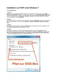
2. Installation
No problem: after the download (http://home.ict.nl/~arivoors/) unzip the package and start the 4NEC2 exe file.
After the successful installation right click on the 4NEC2X – exe file and install this software in the same directory.
The software is completely free and no licensing necessary. Bugs or proposals for improvements can be mailed
to the author Arie Voors who has done a huge work. So tell him „Thank you“ in the mail for his work.
3. Getting Started
Click on the 4NEC2X icon and you get two windows on your screen:
Main
Geometry
(F2) and
(F3)
After the simulation two additional windows can be opened:
Pattern
Impedance / SWR / Gain
(F4) and
(F5).
:
Remarks:
a) Input and property inputs, modifications and start of simulation are all done in the Main window.
b) The antenna geometry is shown in the Geometry window due to the Input NEC File.
c) Far field and near field simulation results are presented in the Pattern window.
d) And finally when sweeping you can see the impedance or the SWR or the F/B ratio versus frequency by
pressing F5.
3

4. Geometry Builder, Geometry Editor or Text Editor to create a NEC File?
This must be decided by the user who has the choice.
a) Creating the NEC file with the Geometry Builder is fine. For Patch-, Plane-, Box-,
Helix-, Spherical-, Cylinder- or Parabolic structures there exist own menus with own screens and the usage is
really simple. But you have only the listed 7 antenna types…
b) To create any desired structure is an affair for the Geometry Editor. This editor this mainly foreseen for
beginners and is easy of use.
The next 3 editors concentrate directly on the NEC file, because this is the goal of all preparation for the
simulation. That needs more effort for the user but gives more options for simulation and optimizing.
But remember:
All length values in a NEC File are always read as „Meters“. Otherwise you must write an additional “GS”
card with a scaling factor for correction (example: entries in Inches…) which is applied to the complete
structure.
But now let’s have a look at the 3 editors:
With a simple text editor like Notepad you have to write the pure NEC file and / or modify entries in it. So the
complete antenna structure must exist in your brain before writing -- but this is the fastest and most effective
way.
That is not difficult and after a short time you are familiar with this method. Then you are able to modify
structures or parts of them in a hurry….
The „old 4NEC2 – Editor“ was a progress because of using buttons to separate the different parts of the NEC
file (but today no longer used and maintained).
e) the „new 4NEC2-Editor“ uses menus with lines and columns for the different entries. Very fine -- but the user
with lot of experience misses now the direct view on the complete NEC file. So after some time of working with
4NEC2 nearly everybody returns to Notepad.....
In the following examples and projects all these different editor methods are demonstrated. So please examine
and decide yourself.
4

5. Starting with the included “example2.nec“ (300MHz Dipole)
5.1. Far Field Simulation
Please change to the folder “models“ and open the “example2.nec” file.
In the left (= Main) window you find the simulation frequency and wavelength (= big red circle). The small red
circle in the under left corner of the window indicates that the dipole is divided into 9 segments. The right window
shows the dipole geometry in the related coordinate system.
Now press the F7 button (= start of calculation) and
choose „Far Field pattern“, “Full“ and “Generate“.
An arc resolution of 5 degrees will do the job for the first
time, giving short calculating times.
Then press “Generate”.
5

This is the success and the main window is now fulfilled with entries and data. Now Press F4 and the vertical
radiation pattern is shown in an additional window.
The „Show“ menu in the Pattern (F4) window offers several options. With “Next pattern” and Previous
pattern” you can walk through the diagrams.
Pressing „Indicator“ gives an additional radial cursor for the diagram. If you
left click on any point of the pattern curve with the mouse the cursor snaps to
this point and the values of this point are indicated.
6

Under “Far Field“ can be found:
a) The switch for changing to the Horizontal Plane.
b) The option to change to the „ARRL-style scale“,
using a logarithmic scaling for the amplitude
including an „automatic scaling spread“. So all lobes
of a pattern are visible without efforts.
c) “Multi Pattern“ shows all diagrams for chosen
polarity.
d) “Bold lines“ gives thick lines of the curves and
e) “Font scaling“ is self explaining.
f) At last you can switch the azimuth angle (Phi) and /
or the elevation angle (Theta) forward or reverse.
The rest of the menu should be tested by yourself.
5.2. Coloured 3D Presentation
This option needs „4NEC2X“. So please start your work in the future always by opening
this program.
Close 4NEC2 and start
4NEC2X
Use again the
„example2.nec“ file and
repeat the far field
simulation. Then select F9
to start the 3D Viewer and
you will get this screen.
Now press the left mouse
button when rolling your
mouse -- this varies the
azimuth and elevation
angle of the diagram
(…for you the result is like
a flight in a helicopter
around the antenna…).
7

Now play a little bit with the following buttons:
a) „Ident“ is used to identify and to mark a desired segment after entering the segment number.
b) „Res“ = “Reset“ to the start position after the invoke of the 3D presentation.
c) “Rotc“ is used to define a segment as rotation centre.
d) „Col“ invokes the colour menu .
Let us continue with the proposed 3D presentation of the antenna’s radiation.
Chose these settings….
…and you get this screen. The pattern can be rotated like before by using the mouse.
8

Here follow some presentations which are of interest for a lot users:
At first the current
distribution on the
antenna wire…
…or additionally the
phase distribution.
Or all the segments of the wire can be made visible:
Play now yourself with this huge amount of possibilities…but this takes time….
9

5.3. Opening the NEC-File with the Notepad Editor
Change to the Main menu (F2), open “settings” and chose notepad-editor. Then press F6 to open the NEC file of
our antenna.
Please do not jump over this chapter, because a deep analysis of the NEC file details helps to modify or
to optimize or to analyse error messages.
Every line starts with a short abbreviation (= card name) and describes in a short form the task of the line.
Attention:
In the main window you find a “NEC short reference“ in the help menu.
Now let us examine every line.
Line 1 and line 2: “CM“ starts a comment line with a maximum of 30 signs.
----------------------------------------------------------------------------------------------------------------------------------------
Line 3:
“CE“ is “End of comment“
-----------------------------------------------------------------------------------------------------------------------------------------
Line 4:
“SY“ stands for a “Symbol“ and this is always a Variable (here: length = len=0.4836).
Caution: all length values in a NEC file are given and calculated in Meters.
Corrections can be made by using an additional “GS” card (= geometry scaling) e.
g. when using feet instead of meters. This scaling factor is applied to the complete
structure.
---------------------------------------------------------------------------------------------------------------------------------------
Line 5:
“GW“ =„Geometry of wire“. Let us have a detailed look at the entries of this line.
The line starts with “1“ (= “Wire number 1“).
“9“ indicates that the wire is divided into 9 Segments.
“0 / -len/2 / 0“ are the xyz coordinates of the wire’s starting point. Length unit is
always “Meter“.
“0 / len/2 / 0“ are the xyz coordinates of the wire’s end point.
“.0001“ is the wire’s radius in Meters.
------------------------------------------------------------------------------------------------------------------------------------
Line 6:
„GE“ = end of “geometry information“, followed by a number which describes the
ground
“0“ means: no ground = free space.
“-1“ or “1“ represent a ground, but the details must be entered in a separate
“Ground card“ (= GN card).
------------------------------------------------------------------------------------------------------------------------------------
10

Line 7:
„LD“ = „Loading of a segment“. Please use the NEC short reference
and the NEC manual in the online help to find out all options.
“5” = in this example only “LD 5“ is used to enter the conductivity of the antenna wire.
“1” = Wire 1.
„0 0“ = two empty fields.
„5.8001E7“ is the conductivity for copper ( in mhos).
----------------------------------------------------------------------------------------------------------
Line 8:
“EX“ = “Exitation“.
“0“ = a voltage source is used for excitation.
“1“ = wire 1 (= tag 1) is excited
“5“ = excited segment of Wire 1.
“0“ = an empty field.
„1 0“ = real and imaginary part of the applied complex voltage (1 + j0).
So in this case a real voltage of 1V is used
----------------------------------------------------------------------------------------------------------
Line 9:
“FR“ = frequency information.
Normally a sweep is used and must be programmed. So some information is necessary
if only a fixed frequency is used:
“0“ = linear frequency sweep (“1“ gives a logarithmic sweep)
“1“ = only one frequency step is foreseen.
“0 0“ = two empty fields.
“300“ = start value of frequency = 300MHz.
“0“ = gives a frequency step width of Null MHz
---------------------------------------------------------------------------------------------------------
Line 10:
“EN“ = end of NEC file
---------------------------------------------------------------------------------------------------------
11

5.4. Using the 4NEC2Editor
Caution:
As already mentioned you have the choice between an old and a new version (…you find them in the
“Settings” of the Main menu).
5.4.1. Working with the old 4NEC2 Editor
No problem, it’s like working with Notepad in a modern environment. But this editor version is obsolete.
-------------------------------------------------------------------------------------------------------------------------------------------------------
5.4.2. The new 4NEC2 Editor
The editor can either be
invoked by pressing
+ or by
opening “Settings” in the
main menu followed by
“Edit / Open Input NEC
File”.
This is the first card named
“Symbols”.
All the used wires and their properties are listed on the next card “Geometry“ (Tag Number / number of
segments / xyz coordinates of wire start and end / radius of wire in Meters).
12

---------------------------------------------------------------------------------------------
On the Source / Load card must be noted that a real voltage source (magnitude = 1V) is connected to Tag 1 /
Segment 5.
(Remember: In the load card “LD” in the true NEC file there was only one entry the value of the conductivity of the
copper for the wire).
13

At last information about frequency and
sweeping must be entered. No problem
for a fixed frequency simulation at
300MHz and a dipole in free space.
----------------------------------------------------------------------------------------------------------------------------------------
5.5. Near Field Simulation
Open main“ (F2) and press “F7“. Then choose “Near Field Pattern“
and “E-Field“ and check the entries. This is the task:
Show the E Field distribution for Y = 0 (= centre of dipole as seen in
the direction of the antenna wire and step
„X“ from -20m to +20m in steps of 1,6m
and
„Z“ from 0 to 50m in steps of 2m.“
This is the simulation result.
Important:
The scaling of the field distribution belongs to an
Input Power of 100W (See the “Settings” menu and
then „Input Power“ for changing)
(Remember:
This power value is also used when simulating the
current distribution on the antenna wire).
14

5.6. Sweeping the SWR and the Input Reflection
Press F2, then „F7. Select “Frequency sweep“.
Enter the sweep range from 295 to 305 MHz in the lower half of the
menu. Use a step width of 0.1MHz.
Select „Ver“ (= Vertical Pattern) and start the Simulation with the button
“Generate“.
Simulation result:
15

6. First own Project: 300MHz Dipole over realistic Ground
6.1. Modification in the NEC-File
The easiest way is to use the NEC file of the last example and to modify it:
a) now the dipole hangs 1m above the ground and
b) a realistic ground shall be used.
At first create a new folder for own projects (e. g. “own_examples“) and in it an additional folder this task
(“dipole_over_ground“). Then copy the NEC file of the last example into this new folder and rename it to
dipole_over_ground.nec
Then start 4NEC2X and select the new 4NEC2 editor in the settings menu. Open the new file
“dipole_over_ground.nec” (by pressing F6).
At first enter in the geometry card the height of the dipole’s start and end point to z = 1m
Then switch to “Freq./Ground”. Select “Real ground“ and “Average“. Let the field “Connect wire for Z = 0 to
ground“ free.
Now open the NEC file with notepad to see the modifications:
16

The entries in the Ground card GN are easy to understand:
„2“ = Sommerfeld Norton Ground.
„13“ = Dielectric constant
„.005“ = Conductivity in mhos/m
17

6.2. Far Field Simulation
This is now a well known procedure: Press F7, select “Far Field Pattern“ and
“Full“, followed by ”Generate“.
That gives this pattern for the „Vertical Plane“.
Press F9 (or the 3D button in the menu bar) and you can see the 3D pattern when using the indicated settings:
18

6.3. Near Field Simulation
No problem: use these settings and at once you get the Electrical
Field Strength around the dipole.
Input power is 100W.
19

6.4. Sweeping the SWR and the Input Reflection
Open this well known F7 menu, select “Frequency sweep“ and
choose a sweep range from 295 to 305MHz with a frequency step of
0.1MHz. Select “Ver” = Vertical and click on “Generate” to start the
simulation.
After the (longer) calculation time we get the result. The only difference to the last chapter is an increase of
1.5MHz of the frequency for minimum reflection
20

7. Second project: 300MHz Dipole using thick wires
7.1. The Thick Wire Problem
In the last examples an ideal and infinite thin wire was used for the
simulation. But in practice the wire radius must be increased to get
some mechanical stability.
When opening “Settings” in the main menu you find in „pre-defined
symbols“ an AWG (= American Wire Gauge) list. .
Choose “#3“ with a diameter of 5.8mm because this gives enough
mechanical stability.
Open the NEC file with the editor, enter this value and save all.
So the Geometry card must now look like in the new 4NEC2 editor:
Caution:
Now you must open
“Others“ to activate the
extended kernel for the
fat wire support!
When checking the NEC file with Notepad you will now find an additional new card:
The card is namend “EK“ (= extended kernel) and in the future this new line can also
be added by hand with the Notepad editor…
(Information: the new 4NEC2 editor adds this line automatically).
21

7.2. Far Field and Near Field Simulation
There are no changes
compared to chapter 6.2
(far field) and to chapter 6.3
(near field for an input
power of 100W)
---------------------------------------------------------------------------------------------------------------------------------------------
7.3. Sweeping the SWR and the Input Reflection
This is the influence of the thick wire: the frequency for minimum reflection has decreased to a value with is
10MHz lower.
-------------------------------------------------------------------------------------------------------------------------------------------------
22

7.4. Sweeping the Antenna Gain
At first repeat the simulation of the vertical radiation pattern (see chapter 7.2.), but with an angle resolution
of 1 degree.
In this diagram the elevation angle for
maximum gain is indicated as Theta =
76 degrees.
In the left lower corner of the diagram
an azimuth angle of 360 degrees is
indicated (this means that we see a
“cut” through the 3D pattern at this
angle).
Press F7 to enter the following options:
a) Frequency sweep
b) “Gain“
c) Angle resolution of 1 degree
d) Sweep from 280 to 310MHz with a step width of 0.2MHz
e) Set Theta to 76 degrees and Phi to 0 degrees
Now press “Generate“.
(Click off the information that in this case no “F/B” data = front to
back data are available. Ignore ist and continue with “Generate”)
After the simulation process we see window F5 with the SWR and the input reflection S11.
23

Select “Show“ and “Forward Gain“ to
get the diagram with gain versus the
frequency.
(And in the lower diagram we see that
the remark “no F/B data available” is
true).
-------------------------------------------------------------------
----------------------------------------------------
7.5. Sweeping the Input Impedance
Open “Show“ and select “Imp / Phase”.
Now the exact value of the resonant frequency can be determined to 291MHz (there X = 0).
And as theory says, the input impedance has a value of 70Ω (= radiation resistance).
24

8. A wonderful toy: the Smith Chart Machine
When a simulation is successfully done a Smith chart symbol is highlighted in the menu bar.
So we repeat the frequency sweep of the SWR and the Input reflection over a frequency range from 270 to
310MHz with a step width of 0.2MHz and press the Smith chart button. This gives the following screen:
The simulated S11 is shown as black coloured curve.
In the right lower corner of the screen you find the actual frequency (here. 270MHz). Use the “right” resp. “left
arrow key” on the keyboard to walk through the simulated frequency range and you will here see the S11 value
for this frequency.
Caution:
The information “Mouse” in the next line shows always the impedance value at the actual mouse cursor
position (….and NOT the converted S11 value of the curve for the simulation frequency). This impedance
is indicated in serial and in parallel form.
Additionally we find a pink curve and a green vector running through the actual point of the S11 curve. The circle
radius gives the S11 magnitude (here: 0.409) and this circle is the way on which we march when a transmission
line is connected to the input of the antenna.
The phase of S11 is indicated by the green vector (..use the scaling on the circumference of the Smith chart).
25

On the left of the Smith chart
some additional information is
indicated (using pink pointers).
Caution:
At first think a horizontal
separating line between
the upper and the lower
nomograms ( = marked
in red colour).
In the upper half you get the
relation between the actual
SWR and the SWR voltage
ratio.
In the lower half the relations
between reflection loss,
return loss (in dB), power
reflection coefficient and
voltage reflection coefficient
are indicated.
In the menu for this presentation you find “Export“ and “Import“.
This can be used to produce a Touchstone file (= S parameter file) for export purpose or data saving. You have
the choice between “magnitude / phase” or “dB” form. Also Z parameter files can be produced and exported.
And, if you want, use this Smith chart machine to read and to present foreign (= imported) Touchstone files.
26

9. Optimizing (Key F12)
What is an antenna design worth without optimizing? This can be done after pressing F12, but some preparation
is always necessary:
Every antenna data (which shall be varied for optimizing) must before in the NEC file be replaced by a
variable with a definite default value.
9.1. Optimizing the Antenna Length (thick wire dipole of chapter 7)
Task:
The resonant frequency of the “thick” dipole (see chapter 7) should be 300MHz. So let us automatically vary the
wire length until only the radiation resistance can be measured at the dipole’s input at 300MHz (and X = 0)
Step 1:
Open the NEC file with Notepad and set the default value of the variable “len” to 0.465m. So this line must now
look like:
SY len=0.465
Step 2:
This is now the NEC file:
CM
Loaded dipole above Sommerfeld ground
CM Thick wire used (#3)
CE
End of comment
SY len=0.465 ' Symbol: Length = 0.465m for WL/2
GW 1 9 0 -len/2 1 0 len/2 1 #3 ' Wire 1, 9 segments, halve wavelength long, 1m above ground,
‘ wire gauge: #3
GE -1 ‘ Geometry data entering finished. Ground used, ends of wires
‘ not connected to ground. GN ground card necessary
LD 5 1 0 0 58000000
' Wire conductivity
GN 2 0 0 0 13 0.005
‘ Sommerfeld ground, er = 13, conductivity = 0.005 mhos / m
EK
‘ Extended wire kernel used.
EX 0 1 5 0 1 0 ' Voltage source (1+j0) at wire 1 segment 5.
FR 0 0 0 0 300 0 ‘ No sweep, frequency = 300MHz
EN
‘ End of NEC file
Step 3:
At first use a frequency sweep of the input impedance from 280 to 320MHz to show the goal of optimization.
27

Step 4:
Press F12 and check whether
“Optimize“ and “Default“ are set
in the upper left corner of the
menu. Then select the variable
(by clicking in the list) which
shall be varied for optimization.
In this example we have only
“len” as variable and this
variable can be activated by a
mouse click on its name. But
check whether “len” now can
be found under “Selected”.
At last we set the goal of
optimization. It is possible to
optimize more but one antenna
property but in this case every
property must be combined with
a figures of merit in % (blue
circle in the figure).
Important:
Right click on the “X-in” window with its entered value of 100% to get
this additional menu. There select “minimize” as optimization goal.
At last press “Start” and wait.
This is the result after 23
seconds and you can
press “OK”
28

In the center of the screen changes something and you have now the
choice between “Resume” and “Update NEC-File”.
Here is the result:
Press “Update NEC-File” to save the necessary modifications. If you now
check the file by opening it with Notepad you will find a new value for
the wire length with “len=0.4697”. So start a new simulation (F7) with
the same frequency sweep as before.
A fine done job!
----------------------------------------------------------------------------------------------------------------------------------------
9.2. Parameter-Sweep
Often it is of interest how some characteristic antenna data (e. g. input impedance) vary not only with frequency
but also with special antenna properties (e.g. height over ground). To get a good overview in this case you can
use the parameter sweep for this purpose. Here comes an example.
Task:
Simulate the input impedance of the thick dipole at f = 300MHz when varying the height over ground
between 0.5m and 1,5m in 20 steps.
Step 1:
Use Notepad to open the NEC file for the following modifications:
a) In the “SY” add an entry for height as a variable with a default value of 1m (hght=1).
b) Replace the value of 1m in the GW card by the variable “hght”.
CM
Example 2 : Loaded dipole above Sommerfeld ground
CM Thick wire used (#3)
CE
End of comment
SY len=0.4697, hght=1 ‘ Symbols: Length = 0.4697m for WL/2, height = 1m
GW 1 9 0 -len/2 hght 0 len/2 hght #3 ' Wire 1, 9 segments, halve wavelength long, 1m
‘ above ground, wire gauge: #3
GE -1 ‘ Geometry data entering finished. Ground used, ends of wires
‘ not connected to ground. GN ground card necessary
LD 5 1 0 0 58000000
' Wire conductivity on “Load” card
GN 2 0 0 0 13 0.005
‘ Sommerfeld ground, er = 13, conductivity = 0.005 Siemens / m
EK
‘ Extended wire kernel used.
EX 0 1 5 0 1 0 ' Voltage source (1+j0) at wire 1 segment 5.
FR 0 0 0 0 300 0 ‘ No sweep, frequency = 300MHz
EN
‘ End of NEC file
29

Step 2:
Press F12 to open the
optimizer menu.
Sweep the height over
ground from 0.5m to
20m using 20 steps at
300MHz.
Step 3:
Start the sweep and wait for the message “End of Sweep”. Then click on “OK”.
F5 opens the access to the impedance, the SWR ratio and the gain.
Use the “Show” menu to get the simulation result for the impedance versus the antenna height over ground.
It is nice to see that the input resistance (= radiation resistance) only varies a little bit at different heights. But the
reactance….
30

9.2.2. Far Field Pattern for different Antenna Heights
This is not very difficult. First open the windows F3 and F4.
F3 is a resume of all simulated patterns. But in F4 only one pattern can be indicated for the choosen height over
ground.
Click on F4 to activate it and use the horizontal Cursor tabs to regard the pattern collection.
(Caution: these are the tabs on the right hand side of your keyboard).
The actual height is indicated in the left upper corner of F4, the actual pattern is up lighted in red colour in F3.
31

10. Third Project: Geometry Builder or Text Editor to design a Helix Antenna?
10.1. Fundamentals of Helix-Antenna Design
(Literature: „ARRL Antenna Book“, chapter 19-5. An excellent book which
must be recommended…)
A helix antenna consists of more but three turns of alumina or copper wire and
constant pitch. This gives a circular polarized radiation in direction of the antenna
axis (in the left illustration: upwards) and an antenna gain of more but 8dBi.
The radiation resistance has a value of approx. 140Ω, if a circumference value of
one wavelength is used. Increasing or decreasing the ratio of circumference and
wavelength alters the radiation resistance in the same manner. So the perfect
matching of the antenna to 50Ω is sometimes heavy work. But one important
advantage is the large usable frequency range with nearly constant gain and
radiation resistance and the circular polarization.
. This antenna shall work over “perfect ground” and so in practice you often find a
metal plate or disc (…or sometimes a little alumina pot!) at the feeding side.
In the Web lot of information and design software for a helix antenna can be found. Especially the Online
Calculator are a real help and easy to use. So let us design a 1600MHz which can not only be used for GPS but
also for Meteosat Weather Satellite Reception with such an Online Calculator (homepage: http:// www.vk2zay /
calculators / helical.php)
From this screen we get the following antenna property collection:
Number of windings (= turns) = 5
Operating frequency = 1600MHz
Beam length = 234.219mm
Pitch (= winding spacing) = 46.844mm
Diameter = 59.643mm
(Wire diameter is 2mm)
32

10.2. Design using the Geometry Builder
Start “main“, then “run“. Select “Geomtry Builder“. Go to the “Helix” card for the necessary entries:
Caution:
Let us use 24 segments per turn.
For a wire diameter of 2mm the
radius is 1mm.
Be aware that 3 different units
(Meters, Centimetres and
Millimetres) are used when
entering data!
Because “Left / Right handed” is
not marked you will automatically
get a left hand circular polarization
of the radiation.
If everything is OK, press “Create”
to create the NEC file, which will
open automatically. But with (5
turns) x (24 segments per turn) =
120 segments it is a little huge…
Save it at once using an adequate
namen (e. g. “helix_01.nec“) and
close the file and the Geometry
Builder.
Go to “Main”, open this NEC file and select “NEC Editor (new)“ in the “Settings” menu. Then press F6.
On the “Geometry Card” you find the entry for 120 segments with the all the coordinates and the wire radius of
0.001m
On the “Source / Load“ card a voltage source must be applied to “Tag 1“ and “Segment 1“ with a real amplitude
of 1V:
The frequency is set to 1600MH. No sweep is used.
We use perfect ground and connect wires for Z=0 to
ground.
33

On the “Others“ card the Fat wire support must be activated.
The last card of the menu is used for comments.
Now it is time to save the finished NEC file.
10.3. Far Field Simulation
Press F7 and start the Far Field simulation. The result is a maximum gain
of 9.34dBi
For better understanding:
Press F9 and you can admire the feeding of the Helix
antenna.
The left end of the first segment is connected to
ground and the voltage source is applied to the
centre of this segment.
10.4. Frequency Sweep of Gain and Impedance
A sweep of the gain from1500 to
1800MHz shows very clear the
promised wide band properties of
a Helix antenna.
The gain starts at 9.2dBi for
1500MHz and rises up to 10dBi at
1800MHz.
34

And also the input resistance (= radiation
resistance) has a constant value of 100Ω in this
frequency range.
10.5. And now the same once more, but with the Notepad-Editor
This is faster but needs some effort. Every line of the NEC file will be analyzed with its task and function:
“CM” is always a comment card,
but the end of the comments must
be marked by “CE”.
-------------------------------------------------------------------------------------------------------------------------------------------------
The “GH“ card (=
geometry of helix)
describes the
complete helix
structure (see the left
illustration.
35