UNCORRECTED PROOF

More documents

Recommendations

Info

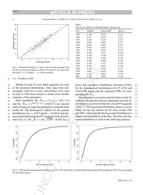
6 J. Brynjarsdóttir, G. Stefánsson / Fisheries Research xxx (2004) xxx–xxx Table 1 The D n test statistics of the Kolmogorov test per year 357 358 359 360 361 362 363 364 365 366 367 368 369 Fig. 2. Scatter plot of log(s 2 j ) vs. log(ȳ j) for every sub-rectangle j that has five or more observations (a total of 241 points). The regression line log(s 2 ) = 2.23 log(ȳ) − 1.6 is also included. 4.2. Goodness of fit Models (4) and (5) were fitted separately for each of the proposed distributions. Only data from subrectangles with five or more observations were used (a total of 1289 observations) to obtain more reliable estimates of the parameters. Both hypothesis H 0 : W yij = Y yji / ˆµ yj ∼G(ˆr, 1/ˆr) and H 0 : W yij = e log(Y yji)−â yj ∼LN(0, ˆb 2 ) are rejected when all data are used and parameters estimated from model (4). The Kolmogorov statistic for the gamma distribution is D n = 0.075 and D n = 0.056 for the lognormal distribution but the 95% quantile of the distribution of D n is 1.36/ √ n = 1.36/ √ 1289 = 0.038. Fig. 3 Year Gamma Log-normal d(n) 0.95 1985 0.106 0.110 0.152 1986 0.121 0.079 0.151 1987 0.103 0.119 0.151 1988 0.093 0.084 0.157 1989 0.104 0.096 0.157 1990 0.095 0.074 0.152 1991 0.105 0.072 0.151 1992 0.103 0.071 0.154 1993 0.104 0.100 0.152 1994 0.109 0.104 0.156 1995 0.100 0.080 0.156 1996 0.142 0.113 0.156 1997 0.129 0.097 0.158 1998 0.105 0.078 0.177 1999 0.087 0.058 0.164 2000 0.113 0.083 0.158 2001 0.138 0.098 0.158 shows the cumulative distribution functions (CDFs) 370 for the hypothesized distributions G(1.07, 0.93) and 371 LN(0,1.05) along with the empirical CDFs of corre- 372 sponding the W yji . 373 The hypothesis can not be rejected when model (5) 374 is fitted to the data for each year separately since the D n 375 test statistics are all lower than the critical 95% quantile 376 (Table 1). The log-normal distribution leads to a lower 377 values for the test statistic for all years except 1985 378 and 1987, indicating that the log-normal distribution is 379 closer to the distribution of the data. Therefore, the log- 380 normal distribution is used in the following analysis. Fig. 3. CDFs for the hypothesized distributions G(1.07, 0.93) and LN(0,1.05) (the thinner lines) along with the empirical CDFs of corresponding W i (the thicker lines). NCORRECTED <strong>PROOF</strong> FISH 1762 1–14
J. Brynjarsdóttir, G. Stefánsson / Fisheries Research xxx (2004) xxx–xxx 7 381 382 383 384 385 386 387 388 389 390 391 392 393 394 395 396 397 398 399 400 401 402 403 404 405 406 407 408 409 410 411 412 413 414 4.3. A stratification model The following model was fitted to log-transformed data: log(Y yji ) = β 0 + α y + β j + γ yj + ɛ yji (8) The parameter β 0 is the intercept (the grand mean), α y is the year effect, β j is the spatial effect of subrectangles and γ yj is the interaction. The errors ɛ i are assumed to be normally distributed with zero mean and constant variance. This is the same model as (4) but in this case all data are used to fit the model (7066 observations). The sub-rectangle factor represents a spatial effect, the effect of the habitation conditions of that area for the cod. These conditions are likely to be controlled by environmental effects such as depth, temperature, amount of food available, etc. The year factor represents the inter-annual fluctuations in the cod stock size and in catchability. This basic model (without interactions) is a fairly standard method of analysis for the purpose of stock assessment. An interaction between sub-rectangles and years represents the difference in variation between sub-rectangles for different years. In other words, the habitation conditions do not change in the same way between years in two different subrectangles. The analysis of variance is shown in Table 2. The terms are added sequentially (first to last). This model accounts for 80.4% of the total variation using 3653/7065 = 51.7% of the total degrees of freedom. Both the main effects of sub-rectangles and years are significant and also the interaction between them. Most of the explained variation comes from the sub-rectangle effect, 49.4%, while the year effect explains only about 3%. The interaction between sub-rectangles and years is a considerable part of the explained variation, 28.2%, but also uses the majority of the total degrees of free- 415 dom of the model. 416 The residuals are plotted to identify model inade- 417 quacy (Fig. 4). A scatter plot of standardized residu- 418 als versus the fitted values shows no obvious structure 419 (Fig. 4a). Residuals plotted against the fitted values 420 indicate that the model does not capture the smallest 421 and largest observations (Fig. 4b). A normal probabil- 422 ity plot of the residuals reveals that the residuals are 423 not normally distributed (Fig. 4c). This is mostly due 424 to the fact that many sub-rectangle/year combinations 425 contain only one observation, resulting in a residual of 426 zero. The standardized residuals plotted against year 427 indicate heterogeneous variability (Fig. 4d). The stan- 428 dard deviations for each year (connected squares in 429 Fig. 4d) are less than unity. The standard deviations for 430 1999–2001 are half those for the other years and the 431 range of residuals for these years is smaller than for 432 the other years. 433 4.4. A continuous model 434 Using sub-rectangles and years as factors does not 435 provide any information or explanation of the data other 436 than the fact that the expected cod catch depends on 437 location and time. A more informative model is one 438 that relates the expected catch to environmental vari- 439 ables that can be expected to effect the behavior of cod 440 on biological grounds. These environmental covariates 441 can be thought of as substitutes for the sub-rectangles 442 effect as they explain why the fish is more likely to be 443 at one place rather than another. 444 The covariates used in the continuous model were 445 selected by looking at box plots of the response ver- 446 sus each of the environmental variables and some of 447 the trawl station data (e.g. Fig. 5). These plots can, of Table 2 Analysis of variance table for the stratification GLM of log-transformed cod catch data Source of variation d.f. SS % expl. SS/d.f. F-test P-value Sub-rectangles 305 8719.4 49.4 28.59 28.14
Page 1 and 2: Fisheries Research xxx (2004) xxx-x
Page 3 and 4: J. Brynjarsdóttir, G. Stefánsson
Page 5: J. Brynjarsdóttir, G. Stefánsson

UNCORRECTED PROOF

You also want an ePaper? Increase the reach of your titles

Delete template?

Save as template?