UNCORRECTED PROOF
UNCORRECTED PROOF
UNCORRECTED PROOF

You also want an ePaper? Increase the reach of your titles
YUMPU automatically turns print PDFs into web optimized ePapers that Google loves.
8 J. Brynjarsdóttir, G. Stefánsson / Fisheries Research xxx (2004) xxx–xxx<br />
448<br />
449<br />
450<br />
451<br />
452<br />
453<br />
454<br />
455<br />
456<br />
457<br />
458<br />
459<br />
460<br />
461<br />
462<br />
463<br />
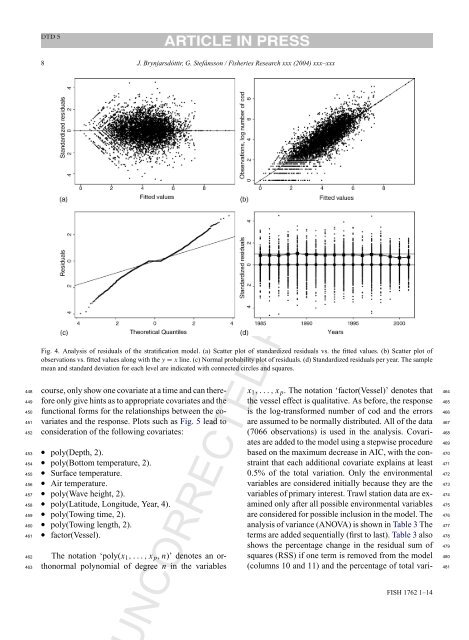
Fig. 4. Analysis of residuals of the stratification model. (a) Scatter plot of standardized residuals vs. the fitted values. (b) Scatter plot of<br />
observations vs. fitted values along with the y = x line. (c) Normal probability plot of residuals. (d) Standardized residuals per year. The sample<br />
mean and standard deviation for each level are indicated with connected circles and squares.<br />
course, only show one covariate at a time and can therefore<br />
only give hints as to appropriate covariates and the<br />
functional forms for the relationships between the covariates<br />
and the response. Plots such as Fig. 5 lead to<br />
consideration of the following covariates:<br />
• poly(Depth, 2).<br />
• poly(Bottom temperature, 2).<br />
• Surface temperature.<br />
• Air temperature.<br />
• poly(Wave height, 2).<br />
• poly(Latitude, Longitude, Year, 4).<br />
• poly(Towing time, 2).<br />
• poly(Towing length, 2).<br />
• factor(Vessel).<br />
The notation ‘poly(x 1 ,...,x p ,n)’ denotes an orthonormal<br />
polynomial of degree n in the variables<br />
x 1 ,...,x p . The notation ‘factor(Vessel)’ denotes that 464<br />
the vessel effect is qualitative. As before, the response 465<br />
is the log-transformed number of cod and the errors 466<br />
are assumed to be normally distributed. All of the data 467<br />
(7066 observations) is used in the analysis. Covari- 468<br />
ates are added to the model using a stepwise procedure 469<br />
based on the maximum decrease in AIC, with the con- 470<br />
straint that each additional covariate explains at least 471<br />
0.5% of the total variation. Only the environmental 472<br />
variables are considered initially because they are the 473<br />
variables of primary interest. Trawl station data are ex- 474<br />
amined only after all possible environmental variables 475<br />
are considered for possible inclusion in the model. The 476<br />
analysis of variance (ANOVA) is shown in Table 3 The 477<br />
terms are added sequentially (first to last). Table 3 also 478<br />
shows the percentage change in the residual sum of 479<br />
squares (RSS) if one term is removed from the model 480<br />
(columns 10 and 11) and the percentage of total vari- 481<br />
NCORRECTED <strong>PROOF</strong><br />
FISH 1762 1–14