Callable Bond/EJ/e

EVALUATION OF CALLABLE BONDS:
FINITE DIFFERENCE METHODS, STABILITY AND ACCURACY ‡
by
HANS-JüRG BüTTLER *
Swiss National Bank
and
University of Zurich
Abstract:
The purpose of this paper is to evaluate numerically the semi-American callable bond by
means of finite difference methods. This study implies three results. First, the numerical error
is greater for the callable bond price than for the straight bond price, and too large for real applications.
This phenomenon can be attributed to the discontinuity in the values of the early redemption
condition. Moreover, many computed prices of the embedded call option turn out to
be negative. Secondly, the numerical accuracy of the callable bond price computed for the relevant
range of interest rates depends entirely on the finite difference scheme which is chosen for
the boundary points. The paper compares the numerical error for four different boundary
schemes, including the one which is extensively used in the finance literature. Thirdly, the
boundary scheme which yields the smallest numerical errror with respect to the straight bond
does not perform best with respect to the callable bond.
Appeared in the Economic Journal, Vol. 105, No. 429, March 1995, 374 – 384.
‡ I thank Karim Abadir (University of Exeter), Jörg Waldvogel (ETH), two anonymous referees and the session
participants of the Royal Economic Society Conference 1994 for valuable comments. An earlier version was
presented at the conference on «Recent Theoretical and Empirical Developments in Finance», University of St.
Gall, Switzerland, 12 – 14 October 1993. A longer version of this paper can be obtained from the author upon
request.
* Mailing address: Swiss National Bank, 8022 Zurich, Switzerland. Phone (direct dialling): +41–1–6313 417,
Fax: +41–1–6313 901.
KEYWORDS: Callable Bonds, Finite Difference Methods, Numerical Accuracy.
JOURNAL OF ECONOMIC LITERATURE CLASSIFICATION: G13.
PAGEHEAD TITLE: Callable Bonds: Finite Difference Methods.

H.-J. Büttler: Callable Bonds: Finite Difference Methods 1
I. INTRODUCTION
The callable bond is a straight (coupon) bond with the provision that allows the debtor to
buy back or to ‘call’ the bond for a specified amount, the call price, plus the accrued interest
since the last coupon date at some time, the call date(s), during the life of the bond. Three types
of callable bonds can be observed in financial markets. The American callable bond may be repurchased
at any time on or before the final redemption day, in contrast to the European or
semi-American counterparts, which may only be called at one or several specific dates, respectively.
In the case of semi-American bonds, the debtor gives the bondholder two months’ notice.
The callable bond can be viewed as a compound security which consists of an otherwise
identical straight bond and of an embedded call option, which is not traded and the price of
which is, therefore, not observable. The embedded call option, which is written on the underlying
straight bond, can be viewed as being ‘sold’ by the initial bondholder to the issuer of the
callable bond, the debtor. Hence, the price of the callable bond must be equal to the price of the
underlying straight bond less the price of the embedded call option at any time.
This paper is motivated by our experience with finite difference methods as well as the
wrong numerical results which have been published in two studies. Gibson-Asner (1990, Table
6, p. 666) reports the computed prices of two almost identical embedded call options for various
points in time. These two options are identical except for the last possible redemption dates
which differ by roughly three months. The prices of these two options with, e. g., approximately
eight years until expiration are reported to be {15.3192, 5.3789}. Our computation indicates
that these two prices differ by 0.2 only. In Leithner (1992, Fig. 5.5, p. 145), the computed
price of the semi-American call option is less than that of the corresponding European call
for small interest rates, but greater for large interest rates. These wrong results presented in
Gibson-Asner and Leithner must be due to numerical errors.
The purpose of this paper is to evaluate numerically the semi-American callable bond by
means of four finite difference methods. As an example, we use the one-factor model of the
(real) term structure of interest rates proposed by Vasicek (1977). The numerical solution of the
finite difference method will be compared with the analytical solution which was derived in
Büttler and Waldvogel (1993a, b).
The outline of the paper is as follows. The next section describes the callable bond price
model. The finite difference methods considered in this paper are explained in the third section,
followed by a section which addresses the question of numerical accuracy of the finite difference
methods. Conclusions are given at the end.
II. THE CALLABLE BOND PRICE MODEL
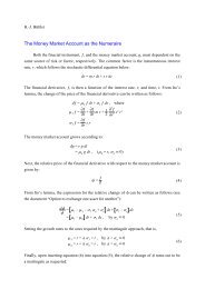
Vasicek (1977) derives the following parabolic partial differential equation to determine
the price of a default-free discount bond, P(r, τ), promising to pay one unit of money on the
maturity day:
P τ
= 1
2 ρ 2 P rr
+ α (γ – r) + ρq P r
– rP, (1)
Royal Economic Society Conference University of Exeter, 28 – 31 March 1994

H.-J. Büttler: Callable Bonds: Finite Difference Methods 2
where the subscripts denote partial derivatives, r the instantaneous interest rate, τ the remaining
time period until the expiration of the discount bond, and q the market price of interest-rate risk
assumed to be constant. If arbitrage opportunities are ruled out, the market price of interest-rate
risk must be the same for all discount bonds of different maturities. Empirically, we would expect
q to be positive. The remaining parameters are those of the underlying interest rate process,
namely the Ornstein-Uhlenbeck process dr = α [γ – r] dt + ρ dz, with α > 0 the speed of adjustment,
γ > 0 the long-run ‘equilibrium’ value of the instantaneous interest rate, t the calendar
time, ρ > 0 the constant instantaneous standard deviation (volatility) of the instantaneous interest
rate, and dz the Gauss-Wiener process.
On the maturity day, the price of the discount bond is equal to one: this is the ‘initial’
condition of (1), noting that ‘time’ τ is measured backwards. The boundary conditions, which
lead to Vasicek’s bond price formula, are given by (i) P(r, τ) → 0 as r → ∞, right boundary
(Brennan and Schwartz, 1977; 1979), and (ii) P(r, τ) = (e – ϑ r ), ϑ > 0, as r → – ∞, left
boundary (Büttler and Waldvogel, 1993a). The right boundary condition says that the price of a
discount bond tends to zero as the instantaneous interest rate grows infinitely large. The left
boundary condition ensures that a particular solution is chosen which grows exponentially at
most as the absolute value of the interest rate becomes very large.
The callable bond satisfies the same partial differential (1) and the same boundary conditions
as the discount bond between the notice dates. On the ‘initial’ day, i. e., the last possible
redemption date, the price of the callable bond is equal to the face value plus the last coupon.
Moreover, the callable bond is subject to the early redemption condition prevailing on each notice
day when the debtor has to decide whether or not to call the bond. The call policy is optimal
if the issuer of the callable bond minimizes his outstanding debt. Therefore, he will call the
bond if the price of the callable bond is greater than the time value of the call price (including the
next coupon). The ‘break-even’ (or critical) interest rate is that interest rate which equates the
price of the callable bond an instant before the notice date (looking backwards in time) and the
time value of the call price. Hence, the price of the callable bond an instant after the notice day
is either equal to the time value of the call price if the actual interest rate is less than the ‘breakeven’
interest rate or equal to the callable bond price an instant before the notice date if the actual
interest rate is greater than the ‘break-even’ interest rate. This is the early redemption condition.
III. FINITE DIFFERENCE METHODS
Four different finite difference methods have been applied to the partial differential equation
(1), namely the explicit method, the implicit method, the Crank-Nicolson method and the
implicit method with a two time-level extrapolation due to Lawson and Morris (1978), henceforth
the Lawson-Morris method. Brennan and Schwartz (1978) have shown that the explicit
method corresponds to the simple binomial model, in contrast to the implicit method which corresponds
to a multinomial model with jumps.
We use Brennan and Schwartz’ (1979) transformation of variables:
Royal Economic Society Conference University of Exeter, 28 – 31 March 1994

H.-J. Büttler: Callable Bonds: Finite Difference Methods 3
x =
1
1 + mr , τ = t – t 0
s – t 0
, (0 ≤ x, τ ≤ 1), F(x, τ) = P(r, t). (2)
Here, m;^ is a scaling factor, s the maximum time until expiration of all the bonds considered,
and τ measures the elapsed time rather than the time to maturity (the differential equation is still
solved backwards in time). The transformed differential equation then becomes (3).
0 =
∂F(x, τ)
∂τ
+ a(x)
∂F(x, τ)
∂x
+ b(x) ∂2 F(x, τ)
∂x 2
+ c(x) F(x, τ), with
a(x) = – (αγ + ρq) m x 2 – α (1 – x) x – ρ 2 m 2 x 3 (s – t 0
) 0,
b(x) = 1
2 ρ 2 m 2 x 4 (1 – x)
(s – t 0
) > 0, c(x) = – (s – t 0
) < 0.
mx
(3)
Two comments are necessary. First, although we consider only non-negative interest rates in
this paper, the transformation (2) allows for a negative interest rate range which is sufficient in
practical applications, for instance, r > –100% for m;^ = 1. In fact, a calculation of the analytical
price of a callable bond with twenty years to expiration and with ten call dates has shown that
the smallest ‘break-even’ interest rate is –13% (Büttler and Waldvogel, 1993b). Secondly, the
numerical error calculated in this paper is based on the analytical price for positive ‘break-even’
interest rates (see footnote 3 of Table 3).
Table 1: Finite Differences for Internal Mesh Points.
Derivative Denominator F i + 1
F i
F i – 1
Equal Interest F x 2 ∆x 1 — – 1
Rate Interval F xx (∆x) 2 1 – 2 1
Unequal Interest F x
∆x + ∆x 0 1 — – 1
Rate Interval F xx
∆x ∆x 0
[∆x + ∆x 0
] 2 ∆x 0
– 2 [∆x + ∆x 0
] 2 ∆x
Comment: Read the second row as F x
= [1·F i + 1
– 1·F i – 1
] / [2 ∆x] and similarly the other rows. ∆x 0
denotes the
interval length to the left of the internal mesh point in question and ∆x the interval length to the right of this
mesh point.
The region of definition of the transformed differential equation, Ω = [0, 1] × [0, 1], is
now divided into meshes. Since we wish to calculate the price of callable bonds for the current
value of the instantaneous interest rate, the meshes are not all of the same size. Moreover, it
might be desirable to have narrow meshes for small interest rates such that the ‘break-even’ interest
rate can be determined with ‘high’ accuracy. Therefore, the x-axis is divided into n 1
equal
intervals between x m
and 1 (equivalently r ∈ [0, r m
]) and n 2
equal intervals between 0 and x m
(equivalently r ∈ [r m
, + ∞]). If n 2
is set equal to zero, then the whole range of positive interest
rates is divided into n 1
equal intervals, possibly except for an initial step at x = 0 (r = ∞). The
current value of the instantaneous interest rate, r 0
, lies always on a mesh point. The steps between
two points in time of interest (e. g., a coupon date and a notice date) will be of equal
length. The mesh points are counted with index i along the x-axis and with index j along the
time axis.
Royal Economic Society Conference University of Exeter, 28 – 31 March 1994

H.-J. Büttler: Callable Bonds: Finite Difference Methods 4
The standard second-order finite differences are applied to (3), namely F τ
= [F j + 1
– F j
] /
∆τ for the partial derivative with respect to time, and those of Table 1 for the partial derivatives
with respect to the interest rate (Smith, 1985; for unequal interest-rate intervals see Schwarz,
1988). For further reference, the mesh ratio is defined to be ψ = ∆τ / (∆x) 2 .
The left boundary condition of the transformed differential equation is F 0 j = 0 for all j. The
right boundary condition of the transformed differential equation (3) is obtained in the following
way. First, note that the transformed differential equation is regular at x = 1, that is, F,
F x
and F xx
are finite at x = 1. Hence, the fourth term of (3) vanishes. Secondly, the partial
derivatives on the right boundary may be approximated by various boundary schemes (Stiefel,
1965; Schwarz, 1988). Unfortunately, these boundary schemes do not have the same local
truncation error as the finite difference approximation at internal mesh points because no points
outside of the region of definition can be taken into account. We tried the five simplest boundary
schemes for i = n (x = 1) which are shown in Table 2. The second boundary scheme is a
complete second-order finite difference approximation. However, it constrains the second partial
derivatives at the points (n, ·) and (n – 1, ·) to be equal. This restriction, which is similar to
the ‘not-a-knot’ condition used for cubic splines (De Boor, 1978), helps to stabilize possible
oscillations. The first boundary scheme, which is extensively used in the finance literature (see,
e. g., Brennan and Schwartz, 1977, 1979; Courtadon, 1982; Duffie, 1992), imposes the same
restriction with respect to the second partial derivative as the second boundary scheme. Moreover,
the first partial derivative of the first boundary scheme applies to the point (n – 1/2, ·)
rather than to the point (n, ·). The third boundary scheme is, in principle, equivalent to the one
for the internal mesh points: the first partial derivative is of the same second order and the second
partial derivatives at the points (n, ·) and (n – 1, ·) are not restricted to be equal. However,
the second partial derivative of this finite difference scheme is now of the third order. The
fourth boundary scheme is of the third order for both partial derivatives, and finally, the fifth
boundary scheme of the fourth order. In summary, none of the five boundary schemes considered
in Table 2 is fully compatible with the finite difference scheme for the internal mesh points.
The choice of one of them is, therefore, at the user’s discretion.
IV. THE ACCURACY OF FINITE DIFFERENCE METHODS
We look first at the stability of the boundary schemes. Numerical experiments for a discount
bond indicate that the first four boundary schemes seem to be stable for all four finite difference
methods considered in this paper, that is, the numerical error shrinks as the meshes get
smaller, holding the mesh ratio constant. However, the fifth boundary scheme seems to be unstable:
the numerical error grows infinitely large (although very slowly) as the meshes get
smaller, holding the mesh ratio constant. This might be due to the fact that the local truncation
error of the fifth boundary scheme is much smaller than that of the internal mesh points. The
fifth boundary scheme is neglected in the following.
Royal Economic Society Conference University of Exeter, 28 – 31 March 1994

H.-J. Büttler: Callable Bonds: Finite Difference Methods 5
It is well known that the explicit mehod is unstable for ‘big’ mesh ratios (Smith, 1985).
Since small mesh ratios require a great deal of time steps, the explicit method is computationally
not efficient. With this respect, the other three finite difference methods considered in this paper
are preferable. Although these three methods are stable for any mesh ratio, they may exhibit
slowly decaying finite oscillations in the neighbourhood of discontinuities in the initial values or
between initial values and boundary values (Smith, 1985). Indeed, our own computations indicate
that oscillations occur after each coupon date of the straight bond for large mesh ratios, especially
with the Crank-Nicolson method. The results to follow refer to the Lawson-Morris
method which performs slightly best.
The numerical accuracy of the finite difference methods under consideration when applied
to the callable bond is rather poor, given a number of interest-rate intervals which is both comparable
with similar problems (Gourlay and Morris, 1980) and computationally feasible. Moreover,
we find that many computed prices of the embedded call option turn out to be negative, in
particular for the third and fourth boundary schemes.
What is the reason for the poor numerical accuracy or the negative prices? We explain this
phenomenon by the discontinuity in the values of the early redemption condition. A closer look
at the evolution of the price vector of a particular callable bond in time reveals this fact quite impressively.
To bear out this assertion most clearly, we chose a European callable bond, the analytical
price of which can be computed with approximate machine precision (Büttler and Waldvogel,
1993a, b). The European callable bond under consideration has a maximum life of 6.811
years until the final expiration date and bears an annual coupon of 7%. Proceeding backwards
in time, we stop the calculation for the first time an instant before the notice day and look at the
numerical error of the callable bond as shown in Fig. 1. The instantaneous interest rate ranges
between zero and 200% in the panel (a). The same function is shown in the panel (b) in a magnified
mode for interest rates between zero and 15%. One time step after the notice day, the
numerical error has a spike at the ‘break-even’ interest rate as shown in Fig. 2. Although this
spike broadens and spreads out over the next few time steps, it introduces slowly decaying finite
oscillations which amplify the numerical error of the callable bond compared with that of
the underlying straight bond as shown in Fig. 3 – 5. We conclude that the difference in accuracy
between the callable bond and its underlying straight bond is entirely due to the discontinuity
in the values of the early redemption condition. The numerical errors for a small sample of
exchange-traded callable bonds are shown in Table 3.
V. CONCLUSIONS
This study implies three results. First, the numerical error is greater for the callable bond
price than for the straight bond price, and too large for real applications which require a twodigit
accuracy at least. This phenomenon can be attributed to the discontinuity in the values of
the early redemption condition. Moreover, many computed prices of the embedded call option
turn out to be negative. The phenomenon of negative computed prices of the embedded call op-
Royal Economic Society Conference University of Exeter, 28 – 31 March 1994

H.-J. Büttler: Callable Bonds: Finite Difference Methods 6
tion has also been observed, but has not been explained, in Gibson-Asner (1990, p. 670). In an
empirical study, Longstaff (1992) finds that ‘nearly two-thirds of the call values implied by a
sample of recent callable bond prices are negative.’ Our own computations indicate that all but
two call option prices implied by the sample of Table 3 are negative. We argue that the negative
computed or implied prices of the embedded call option might be due to the numerical error of
the finite difference methods under consideration.
Secondly, the numerical accuracy of the callable bond price computed for the relevant
range of interest rates depends entirely on the finite difference scheme which is chosen for the
boundary points (see Fig. 1 – 5).
Thirdly, the boundary scheme which yields the smallest numerical errror with respect to
the straight bond does not perform best with respect to the callable bond. The boundary scheme
#4 has the smallest root mean square error with respect to the underlying straight bond for the
sample of Table 3, in contrast to the boundary scheme #2 which has the smallest root mean
square error with respect to the callable bond. Since, in general, you do not know the analytical
solution of the partial differential equation in question, you would probably choose that boundary
scheme which gives you the smallest numerical error with respect to a similar security with
a known analytical solution, that is, the straight bond. However, this choice is misleading.
REFERENCES
Brennan, M. J. and Schwartz, E. S. (1977). ‘Savings Bonds, Retractable Bonds and Callable Bonds’, Journal of Financial
Economics, vol. 5, pp. 67 – 88.
Brennan, M. J. and Schwartz, E. S. (1978). ‘Finite Difference Methods and Jump Processes Arising in the Pricing of
Contingent Claims: A Synthesis’, Journal of Financial and Quantitative Analysis, vol. 13, pp. 461 – 474.
Brennan, M. J. and Schwartz, E. S. (1979). ‘A Continuous Time Approach to the Pricing of Bonds’, Journal of Banking
and Finance, vol. 3, pp. 133 – 155.
Büttler, H.-J. and Waldvogel, J. (1993a). ‘Pricing the European and Semi-American Callable Bond by means of Series
Solutions of Parabolic Differential Equations’, mimeo, Swiss National Bank.
Büttler, H.-J. and Waldvogel, J. (1993b). ‘Numerical Evaluation of Callable Bonds Using Green’s Function’, mimeo,
Swiss National Bank.
Courtadon, G. (1982). ‘The Pricing of Options on Default-free Bonds’, Journal of Financial and Quantitative Analysis,
vol. XVII, pp. 75 – 101.
De Boor, C. (1978). A Practical Guide to Splines, New York: Springer-Verlag.
Duffie, D. (1992). Dynamic Asset Pricing Theory, Princeton (N. J.): Princeton University Press.
Gibson-Asner, R. (1990). ‘Valuing Swiss Default-free Callable Bonds’, Journal of Banking and Finance, vol. 14, pp.
649 – 672.
Gourlay, A. R. and Morris, J. Ll. (1980). ‘The Extrapolation of First Order Methods for Parabolic Partial Differential
Equations, II’, SIAM Journal of Numerical Analysis, vol. 17 (no. 5), pp. 641 – 655.
Jensen, K. and Wirth, N. (1982). Pascal: User Manual and Report, New York: Springer-Verlag, second edition.
Lawson, J. D. and Morris, J. Ll. (1978). ‘The Extrapolation of First Order Methods for Parabolic Partial Differential
Equations, I’, SIAM Journal of Numerical Analysis, vol. 15 (no. 7), pp. 1212 – 1224.
Leithner, S. (1992). Valuation and Risk Management of Interest Rate Derivative Securities, Bern: Verlag Paul Haupt.
Longstaff, F. (1992). ‘Are Negative Option Prices Possible? The Callable U. S. Treasury-Bond Puzzle’, Journal of Business,
vol. 65, pp. 571 – 592.
Press, W. H., Flannery, B. P., Teukolsky, S. A. and Vetterling, W. T. (1989). Numerical Recipes in Pascal: The Art of
Scientific Computing, Cambridge (Mass.): Cambridge University Press.
Smith, G. D. (1985). Numerical Solution of Partial Differential Equations: Finite Difference Methods, Oxford: Clarendon
Press, third edition.
Schwarz, H. R. (1988). Numerische Mathematik, Stuttgart: B. G. Teubner, second edition.
Stiefel, E. (1965). Einführung in die numerische Mathematik, Stuttgart: B. G. Teubner.
Vasicek, O. (1977). ‘An Equilibrium Characterization of the Term Structure’, Journal of Financial Economics, vol. 5,
pp. 177 – 188.
Royal Economic Society Conference University of Exeter, 28 – 31 March 1994

H.-J. Büttler: Callable Bonds: Finite Difference Methods 7
Table 3: Price of Callable Bonds Belonging to ‘Bond Baskets’ of the SWISS NATIO-
NAL BANK and Numerical Error of Finite Difference Methods. 1
Number Name of Security Years Number Call Price of Callable Bond
of to of Call Condi- Analy- Finite Difference Method
Security Maturity 2 Dates 3 tion 4 tical 5 #1 #2
Col. 1 Col. 2 Col. 3 Col. 4 Col. 5 Col. 6 Col. 7 Col. 8
16 310 4 1/2% Bern 1986–1998 6.547 2 (1) A 84.57 81.41 82.60
16 242 4 1/4% Bern 1987–1999 7.519 2 (1) A 82.55 79.54 80.75
16 506 5 1/4% Graub. 89–1999 7.728 2 (2) A 85.67 85.23 86.34
17 459 4 1/4% Waadt 1986–1998 6.269 2 (1) A 83.66 80.38 81.58
17 360 4 1/4% Wallis 1986–1998 6.478 2 (1) A 83.45 80.20 81.41
17 364 7% Wallis 1990–2000 8.811 2 (2) A 95.68 91.39 93.04
17 610 6 1/2% Zürich 1991–2001 9.322 2 (2) A 93.17 93.90 90.59
15 461 4 3/4% Eidg. 1986–2001 9.036 5 (1) B 84.63 82.30 83.38
15 710 4 1/4% Eidg. 1986–2001 9.292 5 (1) B 81.32 78.94 80.04
15 712 4 1/4% Eidg. 1986–2011 19.942 10 (1) C 76.76 78.63 78.40
15 718 4 1/4% Eidg. 1987–2012 20.172 10 (1) C 76.67 78.62 78.37
15 722 4% Eidg. 1988–1999 7.117 3 (1) D 81.63 78.43 79.67
15 726 4 1/4% Eidg. 1989–2001 9.050 4 (1) E 81.50 79.02 80.14
15 736 5 1/2% Eidg. 1989–1998 6.819 2 (2) A 86.96 86.49 87.59
15 738 5 1/2% Eidg. 1990–1999 7.042 2 (2) A 86.98 86.54 87.64
15 740 6 1/4% Eidg. 1990–2000 8.208 2 (2) A 91.05 91.33 92.34
15 745 6 1/2% Eidg. 1990–2000 8.378 2 (2) A 92.49 92.97 89.60
15 227 6 1/2% Eidg. 1990–1999 7.564 2 (2) A 91.93 92.23 88.82
15 747 6 3/4% Eidg. 1991–2001 9.081 2 (2) A 94.50 91.95 91.83
15 749 6 1/4% Eidg. 1991–2001 9.228 2 (2) A 91.62 92.18 93.12
15 751 6 1/4% Eidg. 1991–2003 11.400 4 (2) E 92.87 94.12 91.89
15 753 6 1/4% Eidg. 1991–2002 10.561 2 (2) A 92.39 93.36 94.17
1 Trading day 23 December 1991. Given the current value of the instantaneous interest rate and three observed
continuous-time discount bond yields {0.075228, 0.07753, 0.06647, 0.06298} with {0, 1.0, 7.175, 10.25} years
until expiration, the parameters of Vasicek’s theoretical yield curve have been estimated by means of a modified
Newton-Raphson algorithm. The underlying interest-rate process is the Ornstein-Uhlenbeck process dr = α (γ –
r) dt + ρ dz, where r is the instantaneous interest rate and dz the Gauss-Wiener process. The estimated parameters
of the term structure are: the speed of adjustment α = 0.4418, the long-run ‘equilibrium’ value of the instantaneous
interest rate γ = 0.03485 [discrete-time equivalent 3.546% p. a.], the volatility of the instantaneous interest
rate ρ = 0.1326, and the market price of interest-rate risk q = 0.2117. The instantaneous interest rate has been
approximated by the tomorrow-next rate; it was r 0
= 0.075228 [discrete-time equivalent 7.813% p. a.] on the
trading day in question. The bonds in the upper panel have been issued by cantons, those in the lower panel by
the Swiss confederation.
2 Maximum time period until maturity.
3 The numbers in brackets denote the numbers of positive ‘break-even’ interest rates. These numbers have been
employed to compute the analytical prices for this Table because the finite difference methods are applied to the
partial differential equation with non-negative interest rates only.
4 Call condition type A: the call price is equal to 100 at both call dates. Call condition type B: the first call
price (when moving forwards in time) is equal to 101.5; annual reduction of 0.5 percentage points until 100.
Call condition type C: the first call price (when moving forwards in time) is equal to 102.5; annual reduction of
0.5 percentage points until 100. Call condition type D: the first call price (when moving forwards in time) is
equal to 100.5; annual reduction of 0.5 percentage points until 100. Call condition type E: the first call price
(when moving forwards in time) is equal to 101; annual reduction of 0.5 percentage points until 100. There is a
notice period of two months for all call conditions.
Royal Economic Society Conference University of Exeter, 28 – 31 March 1994

H.-J. Büttler: Callable Bonds: Finite Difference Methods 8
Table 3: Continued. Price of Callable Bonds Belonging to ‘Bond Baskets’ of the
SWISS NATIONAL BANK and Numerical Error.
Number Name of Security Price of Callable Bond Percentage Error of Finite Difference Method
of with Bound. Scheme #… 6 Boundary Scheme
Security #3 #4 #1 7 #2 8 #3 9 #4 10
Col. 1 Col. 2 Col. 9 Col. 10 Col. 11 Col. 12 Col. 13 Col. 14
16 310 4 1/2% Bern 1986–1998 92.84 91.12 – 3.7 – 2.3 + 9.8 + 7.7
16 242 4 1/4% Bern 1987–1999 91.27 89.43 – 3.6 – 2.2 + 10.6 + 8.3
16 506 5 1/4% Graub. 89–1999 95.16 93.48 – 0.5 + 0.8 + 11.1 + 9.1
17 459 4 1/4% Waadt 1986–1998 92.19 90.46 – 3.9 – 2.5 + 10.2 + 8.1
17 360 4 1/4% Wallis 1986–1998 92.06 90.30 – 3.9 – 2.4 + 10.3 + 8.2
17 364 7% Wallis 1990–2000 103.10 101.74 – 4.5 – 2.8 + 7.8 + 6.3
17 610 6 1/2% Zürich 1991–2001 100.85 99.46 + 0.8 – 2.8 + 8.2 + 6.7
15 461 4 3/4% Eidg. 1986–2001 96.79 94.35 – 2.8 – 1.5 + 14.4 + 11.5
15 710 4 1/4% Eidg. 1986–2001 95.33 92.71 – 2.9 – 1.6 + 17.2 + 14.0
15 712 4 1/4% Eidg. 1986–2011 91.08 88.62 + 2.4 + 2.1 + 18.7 + 15.4
15 718 4 1/4% Eidg. 1987–2012 90.77 88.36 + 2.5 + 2.2 + 18.4 + 15.2
15 722 4% Eidg. 1988–1999 92.91 90.72 – 3.9 – 2.4 + 13.8 + 11.1
15 726 4 1/4% Eidg. 1989–2001 94.32 91.74 – 3.0 – 1.7 + 15.7 + 12.6
15 736 5 1/2% Eidg. 1989–1998 96.21 94.61 – 0.5 + 0.7 + 10.6 + 8.8
15 738 5 1/2% Eidg. 1990–1999 96.25 94.63 – 0.5 + 0.8 + 10.7 + 8.8
15 740 6 1/4% Eidg. 1990–2000 99.39 97.88 + 0.3 + 1.4 + 9.2 + 7.5
15 745 6 1/2% Eidg. 1990–2000 100.54 99.08 + 0.5 – 3.1 + 8.7 + 7.1
15 227 6 1/2% Eidg. 1990–1999 100.16 98.69 + 0.3 – 3.4 + 8.9 + 7.3
15 747 6 3/4% Eidg. 1991–2001 102.05 100.68 – 2.7 – 2.8 + 8.0 + 6.5
15 749 6 1/4% Eidg. 1991–2001 99.58 98.14 + 0.6 + 1.6 + 8.7 + 7.1
15 751 6 1/4% Eidg. 1991–2003 102.09 99.99 + 1.3 – 1.1 + 9.9 + 7.7
15 753 6 1/4% Eidg. 1991–2002 99.67 98.37 + 1.1 + 1.9 + 7.9 + 6.5
Root Mean Square Error for the Callable Bonds 2.6 2.1 11.8 9.6
Root Mean Square Error for the Underlying Straight Bonds 11 1.8 1.5 1.2 0.9
5 Price obtained from the analytical solution by means of numerical quadrature involving Green’s function
(Büttler and Waldvogel, 1993a, b) minus the accrued interest since the last coupon date. See footnote 3. All the
digits displayed are correct (the accuracy is almost equal to the machine precision).
6 Price obtained from the numerical solution of the partial differential equation by means of the Lawson-Morris
method minus the accrued interest since the last coupon date. The parameters of the finite difference method are:
n 1
= 50, n 2
= 50, ψ = 200, s = 10, m;^ = 1, and r m
= 0.15. Actually, the computer program modifies slightly
these parameters as described in the longer version of this paper. The computer program has been written in PAS-
CAL (Jensen and Wirth, 1978) and runs on the APPLE® MACINTOSH family, the machine precision of which
is 19 – 20 decimal digits (mantissa of the floating-point form). The tridiagonal matrix algorithm of Press et al.
(1989) has been applied to the resulting equation system of the four finite difference methods under consideration.
7 Percentage deviation: (col. 7 / col. 6 – 1) * 100.
8 Percentage deviation: (col. 8 / col. 6 – 1) * 100.
9 Percentage deviation: (col. 9 / col. 6 – 1) * 100.
10 Percentage deviation: (col. 10 / col. 6 – 1) * 100.
11 The analytical price of the underlying straight bond has been obtained from Vasicek’s bond price model minus
the accrued interest since the last coupon date. The numerical price of the underlying straight bond has been
obtained from the numerical solution of the partial differential equation by means of the Lawson-Morris method
minus the accrued interest since the last coupon date. The parameters of the finite difference method are the same
as those given in footnote 6.
Royal Economic Society Conference University of Exeter, 28 – 31 March 1994

H.-J. Büttler: Callable Bonds: Finite Difference Methods 9
0.00
#3 & #4
0.00
#4
#3
Percentage Error
-0.05
-0.10
#2
#1
Percentage Error
-0.05
-0.10
#2
#1
-0.15
0.0
(a)
0.5
1.0
Interest Rate
1.5
2.0
-0.15
0.00
Fig. 1a & b: Percentage Error on the Notice Day. ‡
(b)
0.05 0.10
Interest Rate
0.15
0.05
0.05
Percentage Error
0.00
-0.05
0.0
#3 & #4
#1 & #2
0.5 1.0
Interest Rate
1.5
(a)
2.0
Percentage Error
0.00
-0.05
0.00
#4
(b)
#2
#3
0.05 0.10
Interest Rate
Fig. 2a & b: Percentage Error One Time Step after the Notice Day. ‡
#1
0.15
3
3
2
2
#3
Percentage Error
1
0
-1
-2
0.0
#3 & #4
#1 & #2
0.5 1.0
Interest Rate
1.5
(a)
2.0
Percentage Error
1
0
-1
-2
0.00
#2
#4
#1
0.05 0.10
Interest Rate
(b)
0.15
Fig. 3a & b: Percentage Error after Two Years. ‡
‡ The numbers refer to the boundary schemes of Table 2. The parameters of the Lawson-Morris method are n 1
= 50, r m = 0.15, n 2 = 50, ψ = 200, ∆t = 1/74th of a year, s = 10 and m;^ = 1.
Royal Economic Society Conference University of Exeter, 28 – 31 March 1994

H.-J. Büttler: Callable Bonds: Finite Difference Methods 10
Percentage Error
5
4
3
2
1
0
-1
#4
#2
#3
Percentage Error
5
4
3
2
1
0
-1
#4
#2
#3
(b)
-2
-3
0.0
#1
0.5 1.0
Interest Rate
1.5
(a)
2.0
-2
-3
0.00
#1
0.05
Interest Rate
0.10
0.15
Fig. 4a & b: Percentage Error after 6.811 Years. ‡
0.8
0.8
Percentage Error
0.6
0.4
0.2
0.0
-0.2
-0.4
-0.6
-0.8
0.0
#3
#2
#4
0.5 1.0
Interest Rate
#1
1.5
(a)
2.0
Percentage Error
0.6
0.4
0.2
0.0
-0.2
-0.4
-0.6
-0.8
0.00
#4
#3
0.05
Interest Rate
Fig. 5a & b: Percentage Error of the Underlying Straight Bond. ‡
#1
#2
0.10
(b)
0.15
Table 2: Five Boundary Schemes.
Scheme # Derivative Denominato F n
F n – 1
F n – 2
F n – 3
F n – 4
r
1 F x ∆x 1 – 1 — — —
F xx (∆x) 2 1 – 2 1 — —
2 F x 2 ∆x 3 – 4 1 — —
F xx (∆x) 2 1 – 2 1 — —
3 F x 2 ∆x 3 – 4 1 — —
F xx (∆x) 2 2 – 5 4 – 1 —
4 F x 6 ∆x 11 – 18 9 – 2 —
F xx (∆x) 2 2 – 5 4 – 1 —
5 F x 12 ∆x 25 – 48 36 – 16 3
F xx 12 (∆x) 2 35 – 104 114 – 56 11
‡ The numbers refer to the boundary schemes of Table 2. The parameters of the Lawson-Morris method are n 1
= 50, r m = 0.15, n 2 = 50, ψ = 200, ∆t = 1/74th of a year, s = 10 and m;^ = 1.
Royal Economic Society Conference University of Exeter, 28 – 31 March 1994

H.-J. Büttler: Callable Bonds: Finite Difference Methods 11
Comment: Read the second row as F x
= [1·F n
– 1·F n – 1
] / ∆x and similarly the other rows.
Royal Economic Society Conference University of Exeter, 28 – 31 March 1994