Callable Bond/EJ/e

More documents

Recommendations

Info

H.-J. Büttler: Callable Bonds: Finite Difference Methods 3 x = 1 1 + mr , τ = t – t 0 s – t 0 , (0 ≤ x, τ ≤ 1), F(x, τ) = P(r, t). (2) Here, m;^ is a scaling factor, s the maximum time until expiration of all the bonds considered, and τ measures the elapsed time rather than the time to maturity (the differential equation is still solved backwards in time). The transformed differential equation then becomes (3). 0 = ∂F(x, τ) ∂τ + a(x) ∂F(x, τ) ∂x + b(x) ∂2 F(x, τ) ∂x 2 + c(x) F(x, τ), with a(x) = – (αγ + ρq) m x 2 – α (1 – x) x – ρ 2 m 2 x 3 (s – t 0 ) 0, b(x) = 1 2 ρ 2 m 2 x 4 (1 – x) (s – t 0 ) > 0, c(x) = – (s – t 0 ) < 0. mx (3) Two comments are necessary. First, although we consider only non-negative interest rates in this paper, the transformation (2) allows for a negative interest rate range which is sufficient in practical applications, for instance, r > –100% for m;^ = 1. In fact, a calculation of the analytical price of a callable bond with twenty years to expiration and with ten call dates has shown that the smallest ‘break-even’ interest rate is –13% (Büttler and Waldvogel, 1993b). Secondly, the numerical error calculated in this paper is based on the analytical price for positive ‘break-even’ interest rates (see footnote 3 of Table 3). 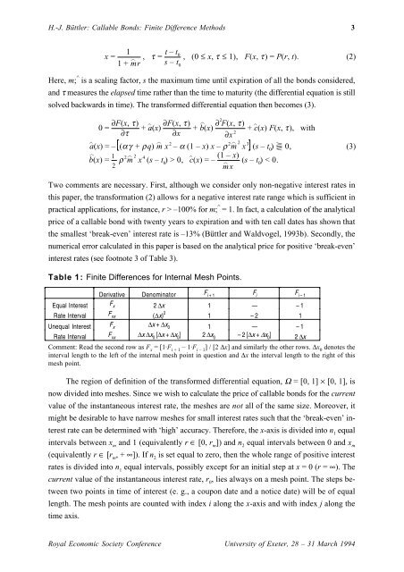Table 1: Finite Differences for Internal Mesh Points. Derivative Denominator F i + 1 F i F i – 1 Equal Interest F x 2 ∆x 1 — – 1 Rate Interval F xx (∆x) 2 1 – 2 1 Unequal Interest F x ∆x + ∆x 0 1 — – 1 Rate Interval F xx ∆x ∆x 0 [∆x + ∆x 0 ] 2 ∆x 0 – 2 [∆x + ∆x 0 ] 2 ∆x Comment: Read the second row as F x = [1·F i + 1 – 1·F i – 1 ] / [2 ∆x] and similarly the other rows. ∆x 0 denotes the interval length to the left of the internal mesh point in question and ∆x the interval length to the right of this mesh point. The region of definition of the transformed differential equation, Ω = [0, 1] × [0, 1], is now divided into meshes. Since we wish to calculate the price of callable bonds for the current value of the instantaneous interest rate, the meshes are not all of the same size. Moreover, it might be desirable to have narrow meshes for small interest rates such that the ‘break-even’ interest rate can be determined with ‘high’ accuracy. Therefore, the x-axis is divided into n 1 equal intervals between x m and 1 (equivalently r ∈ [0, r m ]) and n 2 equal intervals between 0 and x m (equivalently r ∈ [r m , + ∞]). If n 2 is set equal to zero, then the whole range of positive interest rates is divided into n 1 equal intervals, possibly except for an initial step at x = 0 (r = ∞). The current value of the instantaneous interest rate, r 0 , lies always on a mesh point. The steps between two points in time of interest (e. g., a coupon date and a notice date) will be of equal length. The mesh points are counted with index i along the x-axis and with index j along the time axis. Royal Economic Society Conference University of Exeter, 28 – 31 March 1994
H.-J. Büttler: Callable Bonds: Finite Difference Methods 4 The standard second-order finite differences are applied to (3), namely F τ = [F j + 1 – F j ] / ∆τ for the partial derivative with respect to time, and those of Table 1 for the partial derivatives with respect to the interest rate (Smith, 1985; for unequal interest-rate intervals see Schwarz, 1988). For further reference, the mesh ratio is defined to be ψ = ∆τ / (∆x) 2 . The left boundary condition of the transformed differential equation is F 0 j = 0 for all j. The right boundary condition of the transformed differential equation (3) is obtained in the following way. First, note that the transformed differential equation is regular at x = 1, that is, F, F x and F xx are finite at x = 1. Hence, the fourth term of (3) vanishes. Secondly, the partial derivatives on the right boundary may be approximated by various boundary schemes (Stiefel, 1965; Schwarz, 1988). Unfortunately, these boundary schemes do not have the same local truncation error as the finite difference approximation at internal mesh points because no points outside of the region of definition can be taken into account. We tried the five simplest boundary schemes for i = n (x = 1) which are shown in Table 2. The second boundary scheme is a complete second-order finite difference approximation. However, it constrains the second partial derivatives at the points (n, ·) and (n – 1, ·) to be equal. This restriction, which is similar to the ‘not-a-knot’ condition used for cubic splines (De Boor, 1978), helps to stabilize possible oscillations. The first boundary scheme, which is extensively used in the finance literature (see, e. g., Brennan and Schwartz, 1977, 1979; Courtadon, 1982; Duffie, 1992), imposes the same restriction with respect to the second partial derivative as the second boundary scheme. Moreover, the first partial derivative of the first boundary scheme applies to the point (n – 1/2, ·) rather than to the point (n, ·). The third boundary scheme is, in principle, equivalent to the one for the internal mesh points: the first partial derivative is of the same second order and the second partial derivatives at the points (n, ·) and (n – 1, ·) are not restricted to be equal. However, the second partial derivative of this finite difference scheme is now of the third order. The fourth boundary scheme is of the third order for both partial derivatives, and finally, the fifth boundary scheme of the fourth order. In summary, none of the five boundary schemes considered in Table 2 is fully compatible with the finite difference scheme for the internal mesh points. The choice of one of them is, therefore, at the user’s discretion. IV. THE ACCURACY OF FINITE DIFFERENCE METHODS We look first at the stability of the boundary schemes. Numerical experiments for a discount bond indicate that the first four boundary schemes seem to be stable for all four finite difference methods considered in this paper, that is, the numerical error shrinks as the meshes get smaller, holding the mesh ratio constant. However, the fifth boundary scheme seems to be unstable: the numerical error grows infinitely large (although very slowly) as the meshes get smaller, holding the mesh ratio constant. This might be due to the fact that the local truncation error of the fifth boundary scheme is much smaller than that of the internal mesh points. The fifth boundary scheme is neglected in the following. Royal Economic Society Conference University of Exeter, 28 – 31 March 1994
Page 1 and 2: EVALUATION OF CALLABLE BONDS: FINIT
Page 3: H.-J. Büttler: Callable Bonds: Fin
Page 7 and 8: H.-J. Büttler: Callable Bonds: Fin

Callable Bond/EJ/e

Create successful ePaper yourself

Delete template?

Save as template?