Callable Bond/EJ/e
Callable Bond/EJ/e
Callable Bond/EJ/e

You also want an ePaper? Increase the reach of your titles
YUMPU automatically turns print PDFs into web optimized ePapers that Google loves.
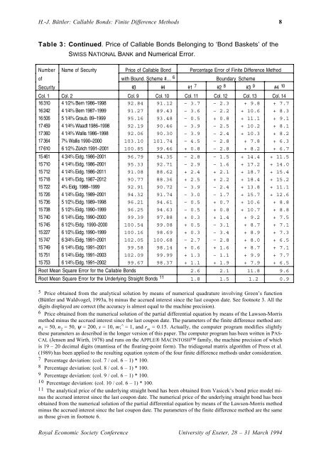
H.-J. Büttler: <strong>Callable</strong> <strong>Bond</strong>s: Finite Difference Methods 8<br />
Table 3: Continued. Price of <strong>Callable</strong> <strong>Bond</strong>s Belonging to ‘<strong>Bond</strong> Baskets’ of the<br />
SWISS NATIONAL BANK and Numerical Error.<br />
Number Name of Security Price of <strong>Callable</strong> <strong>Bond</strong> Percentage Error of Finite Difference Method<br />
of with Bound. Scheme #… 6 Boundary Scheme<br />
Security #3 #4 #1 7 #2 8 #3 9 #4 10<br />
Col. 1 Col. 2 Col. 9 Col. 10 Col. 11 Col. 12 Col. 13 Col. 14<br />
16 310 4 1/2% Bern 1986–1998 92.84 91.12 – 3.7 – 2.3 + 9.8 + 7.7<br />
16 242 4 1/4% Bern 1987–1999 91.27 89.43 – 3.6 – 2.2 + 10.6 + 8.3<br />
16 506 5 1/4% Graub. 89–1999 95.16 93.48 – 0.5 + 0.8 + 11.1 + 9.1<br />
17 459 4 1/4% Waadt 1986–1998 92.19 90.46 – 3.9 – 2.5 + 10.2 + 8.1<br />
17 360 4 1/4% Wallis 1986–1998 92.06 90.30 – 3.9 – 2.4 + 10.3 + 8.2<br />
17 364 7% Wallis 1990–2000 103.10 101.74 – 4.5 – 2.8 + 7.8 + 6.3<br />
17 610 6 1/2% Zürich 1991–2001 100.85 99.46 + 0.8 – 2.8 + 8.2 + 6.7<br />
15 461 4 3/4% Eidg. 1986–2001 96.79 94.35 – 2.8 – 1.5 + 14.4 + 11.5<br />
15 710 4 1/4% Eidg. 1986–2001 95.33 92.71 – 2.9 – 1.6 + 17.2 + 14.0<br />
15 712 4 1/4% Eidg. 1986–2011 91.08 88.62 + 2.4 + 2.1 + 18.7 + 15.4<br />
15 718 4 1/4% Eidg. 1987–2012 90.77 88.36 + 2.5 + 2.2 + 18.4 + 15.2<br />
15 722 4% Eidg. 1988–1999 92.91 90.72 – 3.9 – 2.4 + 13.8 + 11.1<br />
15 726 4 1/4% Eidg. 1989–2001 94.32 91.74 – 3.0 – 1.7 + 15.7 + 12.6<br />
15 736 5 1/2% Eidg. 1989–1998 96.21 94.61 – 0.5 + 0.7 + 10.6 + 8.8<br />
15 738 5 1/2% Eidg. 1990–1999 96.25 94.63 – 0.5 + 0.8 + 10.7 + 8.8<br />
15 740 6 1/4% Eidg. 1990–2000 99.39 97.88 + 0.3 + 1.4 + 9.2 + 7.5<br />
15 745 6 1/2% Eidg. 1990–2000 100.54 99.08 + 0.5 – 3.1 + 8.7 + 7.1<br />
15 227 6 1/2% Eidg. 1990–1999 100.16 98.69 + 0.3 – 3.4 + 8.9 + 7.3<br />
15 747 6 3/4% Eidg. 1991–2001 102.05 100.68 – 2.7 – 2.8 + 8.0 + 6.5<br />
15 749 6 1/4% Eidg. 1991–2001 99.58 98.14 + 0.6 + 1.6 + 8.7 + 7.1<br />
15 751 6 1/4% Eidg. 1991–2003 102.09 99.99 + 1.3 – 1.1 + 9.9 + 7.7<br />
15 753 6 1/4% Eidg. 1991–2002 99.67 98.37 + 1.1 + 1.9 + 7.9 + 6.5<br />
Root Mean Square Error for the <strong>Callable</strong> <strong>Bond</strong>s 2.6 2.1 11.8 9.6<br />
Root Mean Square Error for the Underlying Straight <strong>Bond</strong>s 11 1.8 1.5 1.2 0.9<br />
5 Price obtained from the analytical solution by means of numerical quadrature involving Green’s function<br />
(Büttler and Waldvogel, 1993a, b) minus the accrued interest since the last coupon date. See footnote 3. All the<br />
digits displayed are correct (the accuracy is almost equal to the machine precision).<br />
6 Price obtained from the numerical solution of the partial differential equation by means of the Lawson-Morris<br />
method minus the accrued interest since the last coupon date. The parameters of the finite difference method are:<br />
n 1<br />
= 50, n 2<br />
= 50, ψ = 200, s = 10, m;^ = 1, and r m<br />
= 0.15. Actually, the computer program modifies slightly<br />
these parameters as described in the longer version of this paper. The computer program has been written in PAS-<br />
CAL (Jensen and Wirth, 1978) and runs on the APPLE® MACINTOSH family, the machine precision of which<br />
is 19 – 20 decimal digits (mantissa of the floating-point form). The tridiagonal matrix algorithm of Press et al.<br />
(1989) has been applied to the resulting equation system of the four finite difference methods under consideration.<br />
7 Percentage deviation: (col. 7 / col. 6 – 1) * 100.<br />
8 Percentage deviation: (col. 8 / col. 6 – 1) * 100.<br />
9 Percentage deviation: (col. 9 / col. 6 – 1) * 100.<br />
10 Percentage deviation: (col. 10 / col. 6 – 1) * 100.<br />
11 The analytical price of the underlying straight bond has been obtained from Vasicek’s bond price model minus<br />
the accrued interest since the last coupon date. The numerical price of the underlying straight bond has been<br />
obtained from the numerical solution of the partial differential equation by means of the Lawson-Morris method<br />
minus the accrued interest since the last coupon date. The parameters of the finite difference method are the same<br />
as those given in footnote 6.<br />
Royal Economic Society Conference University of Exeter, 28 – 31 March 1994