R - Fachgebiet Hochspannungstechnik

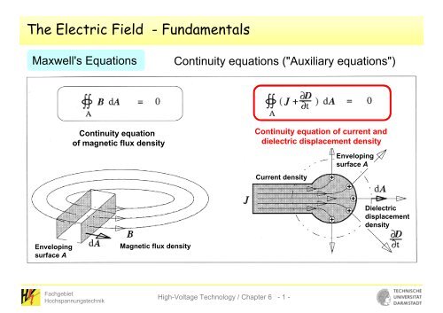
The Electric Field - Fundamentals 

Maxwell's Equations 

Continuity equations ("Auxiliary equations") 

Continuity equation 

of magnetic flux density 

Continuity equation of current and 

dielectric displacement density 

Current density 

Enveloping 

surface A 

Dielectric 

displacement 

density 

Enveloping 

surface A 

Magnetic flux density 

Fachgebiet 

Hochspannungstechnik 

High-Voltage Technology / Chapter 6 - 1 -




Continuity equation of current 

and dielectric displacement 

density: 

∫∫ 

A 

⎛ 

⎜J 

⎝ 

∂D 

⎞ 

+ ⎟dA= 

∂t 

⎠ 

0 

Conversion: 

∫∫ 

A 

∂D d A =− ∫∫ 

J d A = i() 

t 

∂t 

A 

Integration over time: 

∫∫ 

DA d = ∫i() 

t dt = Q 

A 

Gauss's law 

∫∫ DA= d 

A 

Q 







Gauss's law: 

∫∫ DA= d 

A 

Q 

Enveloping 

surface A 

The charge Q equals the integral 

over the spatial charge density η in the 

volume V that is enclosed 

by the enveloping surface. 

Dielectric 

displacement 

density 

∫∫ 

DA d 

A 

= 

∫∫∫ 

V 

ηdV 




Analytical Solution of Gauss's Law 

The electric field of some simple basic geometrical 

configurations (e.g. spherical- or cylindrical-symmetric 

ones), may easily be evaluated by solution of the 

Gauss's law. 

Many of the more complex real configurations in highvoltage 

technology may be referred back to these basic 

configurations. 

DA= d 

Q 

A 

Four-step procedure (sometimes five-step procedure) 





1 st step 

Resolution of Gauss's Law 

∫∫ 

D d A 

A 

= Q 

to the absolute value of D 

Interdependence of charge (that causes the electric field) and 

local distribution of absolute value of electric field strength E = D/ε 





2 nd step 

Evaluating the voltage difference by integration 

of the electric field strength along the path 

U 

21 

1 

= ∫ E ds 

2 

Interdependence of charge Q (that causes the electric field) and 

voltage U: Q = f(U) 





3 rd step 

Evaluating the capacitance of the configuration 

Q 

C = U 





4 th step 

Evaluating the interdependence of electric field strength E 

and voltage U from the results of 1 st and 2 nd step: E = f(U) 





5 th step 

Evaluation of maximum electric field strength E max 

Optimization (e.g. minimization of electrical field strength E max ) 





Sphere in free space 

Point charge with opposite charge at infinity 

Enveloping 

surface A 

D is of same absolute value D(r) at any point 

in space at distance r (for reasons of symmetry) 

Vectors of D and A have the same 

direction at any point in space 

D·dA = D·dA 

Dielectric 

displacement 

density D 

Electric 

field 

strength E 





1 st step 


∫∫ 

D d A 

A 

= Q 


∫∫ 

A 

DA 

2 

d = Dr () ∫∫ 

dA= Dr () ⋅ Ar () = Dr ()4 ⋅ π r = Q 

A 

Dr () = 

Er () = 

Q 

2 

4π 

r 

Q 

4πε 

r 

2 





2 nd step 



U 

21 

1 

2 

ds 

= ∫ E 2 

∞ 

Q 1 Q ⎡ 1⎤ 

Q 

U 

R∞ 

= ∫E() 

r dr = ∫ dr = ⋅ 

4πε r 4πε ⎢ 

− = 

⎣ r⎥⎦ 

4πεR 

R 

∞ 

R 

∞ 

R 

Q = 4πεRU 





3 rd step 


Q 

C = U 

C 

Q 

= = 

U 

4πε 

R 





4 th step 



Q = 4πεRU 

Er () 

= 

Q 

4πεr 

2 

1 

Enveloping 

surface A 

Er () 

R 

= U⋅ 

r 

2 

Dielectric 

displacement 

density D 

Electric 

field 

strength E 

E/E max 

0 

R 

r 





5 th step 



R 

U 

Emax = E( R) 

= U = R 

2 R 

1 

E/E max 

0 

R 

r 




Capacitive Loading by Shielding Electrodes 

Sphere electrode for 1 MV alternating voltage 

Goal: to chose the radius 

such that there are no 

partial discharges. 

Maximum elctric field strength 

on the electrode surface: 

E 

max 

U 

= 

r 

K 

K 





Maximum allowed electric field 

strength in air to achieve freedom 

from partial discharges: 

E max = 25 kV/cm 

Required sphere radius: 

r 

K 

U 

1,4 MV 

K 

= = = 

Emax 

25 kV/cm 

56 cm 





Capacitance of a sphere to ground 

(ground at infinity): 

C K = 4 πε 0 ε r r k 

ε 0 = 8,86 pF/m 

C K = 1,11 r K = 62 pF 

⇒ Capacitive current: 20 mA 

⇒ Reactive power: 20 kVA 





Concentric Spheres (Spheric Capacitor) 

Point charge with opposite charge at infinity 

Enveloping 

surface A 





D·dA = D·dA 





1 st step 


∫∫ 

D d A 

A 

= Q 


∫∫ 

A 

DA 

∫∫ 

2 

d = D() r dA= D() r ⋅ A() r = D()4 

r ⋅ π r = Q 

A 

Dr () = 

Er () = 

Q 

2 

4π 

r 

Q 

4πε 

r 

2 

same procedure as for sphere in free space 





2 nd step 



1 

U 

21 

2 

ds 

= ∫ E Enveloping 

R 

R 

2 2 

2 

Q 1 Q ⎡ 1⎤ 

Q ⎛ 1 1 ⎞ Q R − R 

URR 

= E() 

r dr dr 

1 2 ∫ = ∫ = ⋅ − = ⋅ − = ⋅ 

R 

⎣ ⎦ ⎝ ⎠ 

1 1 

R 

2 1 

2 

4πε r 4πε ⎢ r⎥ ⎜ ⎟ 

R 

4πε R1 R2 4πε 

R 

R 

1⋅ 

R2 

1 

R1⋅ 

R2 

Q = 4πεU ⋅ R − R 

2 1 

surface A 





3 rd step 


Q 

C = U 

Q R1⋅ 

R2 

C = = 4πε 

⋅ U R − R 

2 1 

Gap spacing: s = R 2 - R 1 

s 

Enveloping 

surface A 

C 

= 4πε 

R ⋅ 

1 

s 

+ R 

s 

1 





Concentric spheres 


C 

= 4πε 

R ⋅ 

1 

s 

+ R 

s 

1 

C 

Q 

= = 

U 

4πε 

R 

s 

Enveloping 

surface A 

Enveloping 

surface A 

Dielectric 

displacement 

density D 

Electric 

field 

strength E 

⎛ 

Cconc. = Cfree ⋅ ⎜1+ 

R 

⎝ s 

1 

⎞ 

⎟ 

⎠ 

C conc. always larger than C free 





4 th step 



R1⋅ 

R2 

Q= 4πεU⋅ 

R − R 

2 1 

1 

Er () 

= 

Q 

4πεr 

2 

E/E max 

R 

⋅ R 

1 

1 2 

Er () = U⋅ ⋅ R 

2 

2 

− R 

1 r 

0 

R 

r 





5 th step 



R 

⋅ R 

1 

1 2 

Er () = U⋅ ⋅ R 

2 

2 

− R 

1 r 

1 

E max for r = R 1 

E 

max 

U R2 

= ⋅ 

R R − R 

1 2 1 

E/E max 

0 

R 1 

r 






Spheres in free space 

E 

max 

U R2 

= ⋅ 

R R − R 

1 2 1 

Emax = E( R) 

= 

U 

R 

E 

max 

= E ⋅ 

max, free 

R 

R2 

− R 

2 1 

E max, conc. always larger than E max, free 

Example.... R 2 = 5·R 1 

E max, conc = 1.25·E max, free 

Further example..... 

Transformer shielding sphere 





5 th step 



E 

max 

U R2 

= ⋅ 

R R − R 

1 2 1 

R 1 = 0 

R 1 = R 2 

E max →∞ 

E max →∞ 

(at R 2 unchanged) 

There must be a minimum of maximum field strength! 





5 th step 



Putting the derivative 

∂E 

max 

∂R 

1 

to zero 

...... 

R = 

1, opt 

R 

2 

2 

E 

max, opt 

= 

4U 

R 

2 





E max /E max, min 

Krümmungseffekt 

Abstandseffekt 

E 

max, opt 

= 

4U 

R 

2 

R 1 /R 2 = 0,5 

R 1 /R 2 





5 th step 



Further considerations: 

E 

max 

U R2 

= ⋅ 

R R − R 

1 2 1 

Gap spacing: s = R 2 - R 1 

E 

max 

U R U U 

R R − R R s 

2 

= ⋅ = + 

1 2 1 1 





E 

max 

U R U U 

R R − R R s 

2 

= ⋅ = + 

1 2 1 1 

Maximum electric field strength 

of a sphere in free space 

Electric field strength of an homogeneous 

configuration of gap spacing s 





E 

max 

U R U U 

R R − R R s 

2 

= ⋅ = + 

1 2 1 1 

Curvature effect: 

U U U 

R > → E ≈ 

1 max 

R1 s R1 

• Electric field strength governed by sphere radius 

• Increase of gap spacing of virtually no impact 

on maximum electric field strength 





E 

max 

U R U U 

R R − R R s 

2 

= ⋅ = + 

1 2 1 1 

Distance effect: 

U U U 

R >> s →


E max /E max, min 

Distance- 

Krümmungseffekt 

Curvatureeffect 

Abstandseffekeffect 

R 1 /R 2 = 0,5 0.5 

R 1 /R 2 



High-Voltage Technology / Chapter 6 - 34 - 

l


Configurations similar to "sphere in free space" and 

"concentric sphere"-configuration 

Connector of 

high-voltage leads 

Shielding electrode 

in the corner of an 

high-voltage lab 

Shielding electrode 

in free space 

Elbow of 

a GIS 

Pressurized gas 

capacitor 





Coaxial cylinders 

Coaxial configuration of length z 

Enveloping 

surface A 

Stray effects at the edges neglected 





D·dA = D·dA 





1 st step 


∫∫ 

D d A 

A 

= Q 


∫∫ 

A 

∫∫ 

DA d = Dr () dA= Dr () ⋅ Ar () = Dr ()2 ⋅ π rz= 

Q 

A 

Dr () = 

Er () = 

Q 

2π 

rz 

Q 

2πε 

rz 

similar dependencies as for concentric spheres (but decrease with 1/r) 





2 nd step 



1 

U 

21 

= ∫ E ds 

2 

R 

2 2 

Q 1 Q R2 

Q R 

URR 

= () [ ln ] ln 

1 2 ∫ E r dr = dr r 

R1 

2πε z∫ 

= ⋅ = ⋅ 

r 2πε z 2πε 

z R 

R 

1 1 

R 

R 

2 

1 

Q 

2πε 

z 

= ⋅U 

R2 

ln 

R 

1 

Enveloping 

surface A 





3 rd step 


Q 

C = U 

C 

Q 

= = 

U 

2πε 

z 

R2 

ln 

R 

1 





4 th step 



Q 

2πε 

z 

= ⋅U 

R2 

ln 

R 

1 

Er () 

= 

Q 

2πεrz 

Er () 

= 

r 

U 

⋅ln 

R 

R 

2 

1 





E 

U/R 1 

1 

konzentrische Concentric spheres Kugeln 

Kugel Sphere frei in im free Raum space 

koaxiale Coaxial cylinders Zylinder 


Er () 

R 

= U⋅ 

r 

2 


R 

⋅ R 

1 

1 2 

Er () = U⋅ ⋅ R 

2 

2 

− R 

1 r 

r/R 1 

(R 5·R 1 = 1) (R 2 = 1 ) 

Relative electric field distributions in comparison: sphere in free space, 

concentric spheres, coaxial cylinders 


U 

Er () = 

R2 

r ⋅ln 

R 

1 





5 th step 


Er () = 

U 

r ⋅ln 

R 

2 

R1 

E max for r = R 1 


E 

= E = 

max 1 

R 

1 

U 

⋅ln 

R 

R 

2 

1 





5 th step 



E 

max 1 

R 1 = 0 

= E = 

R 

1 

U 

⋅ln 

R 

R 

2 

1 

E max →∞ 

R 1 = R 2 

E max →∞ 

There must be a minimum of maximum field strength! 





5 th step 



E 

∂Emax 

Putting the derivative to zero ...... 

⎛R 

⎞ 

2 

∂ ⎜ ⎟ 

⎝ R1 

⎠ 

U U R 

= E = = ⋅ 

R 

R1 

⋅ln 

R 

ln 

R 

max 1 

R 

R 

R 

2 1 

2 2 2 

1 1 

u 

v 

What is needed? 

' ' ' 

⎛u⎞ uv − uv 

Quotientenregel : ⎜ ⎟ = 

2 

⎝v 

⎠ v 

d ( ln x)= 

1 

dx 

x 





5 th step 



max 

Putting the derivative to zero ...... 

⎛ R 

⎜ 

⎝ R 

R 

2 

1 

⎞ 

⎟ 

⎠ 

opt 

= e = 

2 

1, opt 2 

∂E 

⎛R 

∂ ⎜ 

⎝ R 

2,718 

Optimized maximum el. field strength: 

R 

= = 0,368⋅R 

Emax, opt 

e 

2 

1 

⎞ 

⎟ 

⎠ 

U U e⋅U 

= = = 

⎛ R ⎞ R 

2 

1, opt 

R2 

R1, opt 

ln ⎜ ⎟ 

⎝ R ⎠ 

1 opt 







E 

max, opt 

4U 

R 

= max, opt 

2 

E 

= 

eU ⋅ 

R 

2 

E max for concentric spheres always larger than for coaxial cylinders 

Reason: Curvature in further dimension of space (z-direction) 





E 1 

E 1, opt R 1 = R 2 /e 

E 1, opt 

R 1 /R 2 

But: û d,max at smaller ratio of radii than 1/e 





Homogeneous field (plate capacitor) 

Stray effects at the edges neglected 

D is of same absolute value D at any point 

of enveloping surface A 



D·dA = D·dA 

Enveloping 

surface A 

s 





1 st step 


∫∫ 

D d A 

A 

= Q 


∫∫ 

A 

∫∫ 

DA d = D dA= D⋅ A= 

Q 

A 

Q 

Dx ( ) = = const. 

A 

Q 

Ex ( ) = = const. 

= E 

ε A 

0 





2 nd step 



1 

U 

21 

= ∫ E ds 

2 

s 

Q s 

U = ⋅ 

∫ E( x) 

dx = E ⋅ s = ε ⋅ A 

0 

Q 

= 

ε ⋅ 

A⋅U 

s 





3 rd step 


Q 

C = U 

Q 

= 

ε ⋅ 

A⋅U 

s 

Q ε ⋅ A 

C = = U s 





4 th step 



Q 

ε ⋅A⋅U 

s 

Q 

Ex ( ) = = const. 

= E 

ε A 

= 

0 

Q U 

Ex ( ) = = = const. 

ε ⋅ A s 





Borda profile (left) and Rogowski profile (right) 





Electric field at the edge of a plate capacitor of Borda profile 




Utilization Factors according to Schwaiger 

Utilization factor 

η = 

E 

E 

0 

max 

Degree of inhomogenity 

1 E 

E 

max 

0 

E 

0 

U 

= 

s 

Electric field of an homogeneous 

configuration of same spacing 

"average electric field strength" 

η = 1 1 

η ≤ 1 

and 

η ≥ , resp. 





η is a function of the geometrical characteristic, i.e. of variables p and q: 

p 

= 

s 

+ 

r 

r 

2r 

2R 

2r 

s 

2r 

s 

2R 

q 

= 

R 

r 

2R 

2r 

s 

q = ∞ 

r ... radius of electrode of more pronounced curvature 

R ... radius of electrode of less pronounced curvature 





Tables ...... 





... or curves 

Spheres 





Breakdown voltage 

Û d = Ê d·s·η 

But..... 

Ê d depends on 

geometry! 

Breakdown electric field strength of air 

at 1013 hPa, 20 °C 

acc. to W. O. Schumann: "Elektrische Durchbruchfeldstärke von 

Gasen", Springer 1923 

for cylinders 

for spheres 

for plates 




Rules for 2D Graphical Electric Field Evaluation 

z: length of configuration 

Field lines and equipotential lines are perpendicular to each other. 






Electrode surface lines are equipotential lines. 





High-voltage potential 

Reference potential 


The potential distribution is given in percentage values. 





ΔU = a·E 


Distance a between two equiquipotential lines is equal to 

always the same potential difference ΔU. 





ΔQ = D·ΔA = ε·E·ΔA = ε·E·b·z 


Distance b between two field lines is equal to 

always the same charge difference ΔQ on the electrode surfaces. 





Rectangular mesh at 

edge lengths a and b 

Capacitance per mesh cell 

at edge lengths a and b: 

ΔQ ε ⋅E⋅b⋅z b 

Δ C = = = ε ⋅z⋅ = const. 

ΔU a⋅E a 


Thus, also b/a = const. 

Appropriate choice: 

b/a = 1 






b/a = 1 

All four edges of a mesh cell must touch inscribed circles. 





Total capacitance: 

np 

C = ⋅Δ C = ε ⋅z⋅ 

n 

s 

n 

n 

p 

s 


n p … number of cells in parallel 

n s … number of cells in series 





Example: Electric field at the edge of a plate capacitor 

Rough approximation of field and potential distribution 






Improved field and potential distribution 






Further improved field and potential distribution

R - Fachgebiet Hochspannungstechnik

You also want an ePaper? Increase the reach of your titles

Delete template?

Save as template?