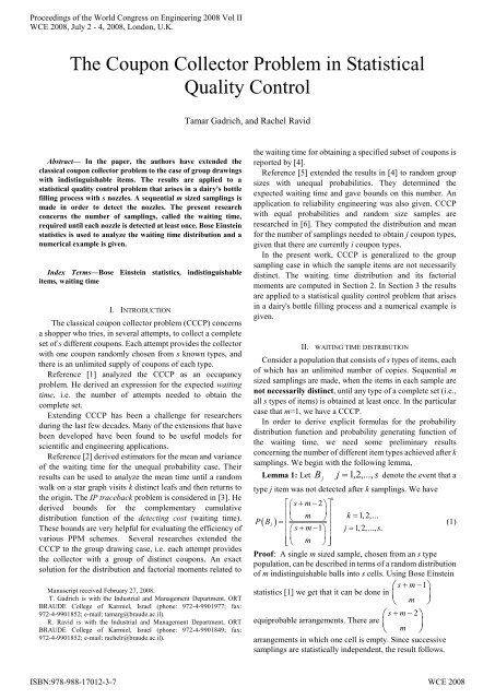
The Coupon Collector Problem in Statistical Quality Control

Proceedings of the World Congress on Engineering 2008 Vol II
WCE 2008, July 2 - 4, 2008, London, U.K.
The Coupon Collector Problem in Statistical
Quality Control
Tamar Gadrich, and Rachel Ravid
Abstract— In the paper, the authors have extended the
classical coupon collector problem to the case of group drawings
with indistinguishable items. The results are applied to a
statistical quality control problem that arises in a dairy's bottle
filling process with s nozzles. A sequential m sized samplings is
made in order to detect the nozzles. The present research
concerns the number of samplings, called the waiting time,
required until each nozzle is detected at least once. Bose Einstein
statistics is used to analyze the waiting time distribution and a
numerical example is given.
Index Terms—Bose Einstein statistics, indistinguishable
items, waiting time
I. INTRODUCTION
The classical coupon collector problem (CCCP) concerns
a shopper who tries, in several attempts, to collect a complete
set of s different coupons. Each attempt provides the collector
with one coupon randomly chosen from s known types, and
there is an unlimited supply of coupons of each type.
Reference [1] analyzed the CCCP as an occupancy
problem. He derived an expression for the expected waiting
time, i.e. the number of attempts needed to obtain the
complete set.
Extending CCCP has been a challenge for researchers
during the last few decades. Many of the extensions that have
been developed have been found to be useful models for
scientific and engineering applications.
Reference [2] derived estimators for the mean and variance
of the waiting time for the unequal probability case. Their
results can be used to analyze the mean time until a random
walk on a star graph visits k distinct leafs and then returns to
the origin. The IP traceback problem is considered in [3]. He
derived bounds for the complementary cumulative
distribution function of the detecting cost (waiting time).
These bounds are very helpful for evaluating the efficiency of
various PPM schemes. Several researches extended the
CCCP to the group drawing case, i.e. each attempt provides
the collector with a group of distinct coupons. An exact
solution for the distribution and factorial moments related to
Manuscript received February 27, 2008.
T. Gadrich is with the Industrial and Management Department, ORT
BRAUDE College of Karmiel, Israel (phone: 972-4-9901977; fax:
972-4-9901852; e-mail: tamarg@braude.ac.il).
R. Ravid is with the Industrial and Management Department, ORT
BRAUDE College of Karmiel, Israel (phone: 972-4-9901849; fax:
972-4-9901852; e-mail: rachelr@braude.ac.il).
the waiting time for obtaining a specified subset of coupons is
reported by [4].
Reference [5] extended the results in [4] to random group
sizes with unequal probabilities. They determined the
expected waiting time and gave bounds on this number. An
application to reliability engineering was also given. CCCP
with equal probabilities and random size samples are
researched in [6]. They computed the distribution and mean
for the number of samplings needed to obtain j coupon types,
given that there are currently i coupon types.
In the present work, CCCP is generalized to the group
sampling case in which the sample items are not necessarily
distinct. The waiting time distribution and its factorial
moments are computed in Section 2. In Section 3 the results
are applied to a statistical quality control problem that arises
in a dairy's bottle filling process and a numerical example is
given.
II. WAITING TIME DISTRIBUTION
Consider a population that consists of s types of items, each
of which has an unlimited number of copies. Sequential m
sized samplings are made, when the items in each sample are
not necessarily distinct, until any type of a complete set (i.e.,
all s types of items) is obtained at least once. In the particular
case that m=1, we have a CCCP.
In order to derive explicit formulas for the probability
distribution function and probability generating function of
the waiting time, we need some preliminary results
concerning the number of different item types achieved after k
samplings. We begin with the following lemma,
Lemma 1: Let B j
j 1,2,...,
s denote the event that a
type j item was not detected after k samplings. We have
k
s m 2
m k 1,2,...
PBj
(1)
sm1
j 1,2,..., s.
m
Proof: A single m sized sample, chosen from an s type
population, can be described in terms of a random distribution
of m indistinguishable balls into s cells. Using Bose Einstein
sm1
statistics [1] we get that it can be done in
m
sm2
equiprobable arrangements. There are
m
arrangements in which one cell is empty. Since successive
samplings are statistically independent, the result follows.
ISBN:978-988-17012-3-7 WCE 2008

Proceedings of the World Congress on Engineering 2008 Vol II
WCE 2008, July 2 - 4, 2008, London, U.K.
Define the random variable X
k
to be the number of different
item types achieved after k samplings;
Theorem 1: The distribution of X k
k 1 is given for
every n (n=1,2,…,s) by:
n
m1
n1
s n
m
k n 1
n s m 1
0
m
P X
P Xk
n 1 1
(2)
k
m
1
n1
s s
1
n
m
(3)
s m 1
0
s
n
m
Proof: Define A j
,...,
( n )
1
j n
to be a fixed n sized
subset of the complete type set. The probability that these
item types will be obtained after k samplings equals:
n
n
j
j
1 1
.
P B 1P B
Using the inclusion-exclusion formula, the probability that
at least one of the item types in A
(n)
will not be obtained in k
samplings is:
P
mn
1
n
n 1
n
1
m
Bj
1
s m 1
1
1
m
Obviously,
n
m1
n 1
s n
m
k
n 1
n
s m 1
0
m
P X
.
Equation (3) is derived from (2) with the aid of Lemma 2 in
[4]. The cumulative distribution function is
k
k
k
.
k k
P X n P X i
s
in
k
s
i
s m 1 s i m i 1
1
m in i 0
m
k
k
s
s
s m 1 m 1
s i
i
1 1
m 0 m imax
, n
i
k
k
s
s
s m 1 s m 1
s
i
1 1
m 0 m imax
, n
i
k
n1
s m 1 s s 1 m 1
n
1
m 0
s n m
k
k
s m 1 s m 1
s
m m
s
1 1 ,
which derived (3).
Corollary 1: The expected number of distinct item types
that are achieved after a series of k 1 samplings is given by
k
ms2
m
E X k
s 1 k 1, 2,...
ms1
m
Proof: For 1 j s define
X
0
I
j
1
item j has not been
obtained during k samplings
otherwise
One can easily see that:
k
s
I
j 1
Clearly,
j
s m 2
m
PI j 1 E I j PBj
1
.
sm1
m
Using the additive property of expectation, we get:
k
sm2
j
j 1
m
s
m
E X k
E I s 1
sm1
.
We now return to our main purpose: determining the
waiting time. Let Z be the number of samplings needed
n
until one collects at least n item types from the complete set.
k
k
k
(4)
ISBN:978-988-17012-3-7 WCE 2008

Proceedings of the World Congress on Engineering 2008 Vol II
WCE 2008, July 2 - 4, 2008, London, U.K.
Theorem 2: The distribution of
(for every k 1) by:
P Z
n
k
Z n
1 n s is given
n1
s s 1
n
1
1
(5)
0
s
n
s m 1
m 1
m 1
m m
m
s m 1 s m 1
k 1
m m
Moreover, the probability generating function (p.g.f.) of
Z is given by
n
G
Zn
n 1 1
1
1
n
s s
(6)
0
s
n
s m 1
m 1
m m s m 1
m 1
m m
Proof: The probability distribution function of Z n can be
obtained from (3) using the following relation:
P Z k P X n P X n .
G
n k k 1
The p.g.f. of
Z
n
Z
E
Z n is defined as:
n
n1
s s 1
k
n
1
1
k 1 0
s
n
(7)
s m 1
m 1
m 1
m m
m
s m 1 s m 1
m m
k 1
m
1
m
Equation (6) follows (7) in the case that
is
s
m1
m
less than 1.
Corollary 2: The p-factorial moments p N
of Z n
are
given by:
1 ... 1
E Z Z Z p
n n n
n1
s s
1
n
1
p! 1
0
s
n
s m 1
m 1
m m
p1
s m 1
m 1
m m
p
Proof: The result in (8) follows (7) by deriving the p.g.f. of
.
Z according to , p times and substituting 1
n
Corollary 3: The expectation and the variance of the
waiting time until we achieve the complete set are given by:
E Z
s1
0
E Z
s
1
s
s1
s
1
s m 1
s
m
s m 1
m 1
m m
(8)
(9)
s
1
(10)
2! 1
0
Z 1
s
s
s m 1
m 1
m m
s m 1
m 1
m m
2
s s s s s
VAR Z E Z Z 1 E Z E Z (11)
Proof: Formulas (9) and (10) are derived from (8) by
substituting p=1 and p=2, respectively; and n=s.
III. NUMERICAL EXAMPLE
The model described in Section II has a direct application
to a statistical quality control problem. Consider a dairy's
bottle filling process consisting of a 24-nozzle machine. After
the bottles are filled with milk, they are gathered in a
collection area. Each hour a random sample of five bottles is
drawn from the collection area and tested in order to control
the filling process. There is no marking on a bottle indicating
which nozzle filled it. The quality engineer wants to know,
after how many hours on the average, bottles filled by any one
of the nozzles will be tested.
Using the notations of Section II, the 24 nozzles form a
2
ISBN:978-988-17012-3-7 WCE 2008

Expectation
Zs
Proceedings of the World Congress on Engineering 2008 Vol II
WCE 2008, July 2 - 4, 2008, London, U.K.
complete set of s types (s=24). An hourly random drawing of
five bottles defines the sample size m=5. Since the bottles are
not marked, the model that assumes that the items in each
sample are not necessarily distinct is suitable here. Using (2),
the probability distribution function of Z
24
is shown in Fig. 1
as a function of k – the number of hourly drawings that are
done in order to test all the nozzles.
0.08
0.07
0.06
0.05
0.04
0.03
0.02
0.01
0
0 5 10 15 20 25 30 35 40 45 50
Time (hours)
Fig. 1. Waiting time probability distribution function for
k=1,2,…,50 (s=24, m=5)
Using (9), the expectation of Z
24
is shown in Fig. 2 as a
function of m – the sample size. This can be useful for the
quality control engineer. If there is any constraint on how
many hourly samplings he can draw, the analyst will easily
find the required sample size for detecting the complete set.
100
90
80
70
60
50
40
30
20
10
0
0 5 10 15 20 25
Sample Size
Fig. 2. Waiting time expectation as a function of the
sample size m (s=24)
In Table 1, for s=24, the expectations and standard
deviations of the waiting time as a function of the sample size
(i.e., as a function of m) are given for the following two cases:
1. In each sampling a set of m different items is drawn. The
factorial moments related to the waiting, in this case, were
obtained in [4] by:
p1
1 ... 1
E Z Z Z p
n n n
s n1
s s j 1
p! 1
m
j0
j s n
nj1
(12)
j s j
m m m
p
The expectation and the standard deviation follow from
(12).
2. In each sampling, a group of m items is drawn, but the
items are not necessarily distinct. The expectation and the
standard deviation can be computed using (9) and (11),
respectively.
Substituting m=1, in (8)-(12) yields the known results for
the CCCP when s=24. On average, one needs around 91
samplings in order to be sure of detecting all 24 different
types.
In the diary problem when m=5; the calculations yield that
on average, after 20 hours all the nozzles will have been
examined.
Table 1. Expectation and standard deviation of the waiting
time s=24
Distinct items Indistinguishable
items
Drawin
g group
Expecta- S.D. Expecta- S.D. size
tion
tion
90.6230 28.8678 90.6230 28.8678 1
44.5973 14.1120 46.4861 14.7463 2
29.2456 9.1909 31.7659 10.0372 3
21.5619 6.7285 24.4002 7.6813 4
16.9449 5.2494 19.9765 6.2667 5
13.8609 4.2618 17.0240 5.3228 6
11.6523 3.5549 14.9123 4.6480 7
9.9905 3.0235 13.3263 4.1413 8
8.6928 2.6088 12.0908 3.7468 9
7.6494 2.2758 11.1008 3.4308 10
6.7906 2.0019 10.2893 3.1719 11
6.0696 1.7721 9.6118 2.9558 12
5.4538 1.5769 9.0374 2.7727 13
4.9195 1.4085 8.5441 2.6156 14
4.4509 1.2589 8.1157 2.4791 15
4.0363 1.1229 7.7400 2.3596 16
3.6632 1.0034 7.4077 2.2539 17
3.3172 0.9058 7.1118 2.1598 18
2.9872 0.8230 6.8464 2.0755 19
2.6745 0.7305 6.6069 1.9995 20
2.3961 0.6008 6.3898 1.9306 21
2.1782 0.4236 6.1919 1.8679 22
2.0435 0.2130 6.0108 1.8105 23
IV. CONCLUSIONS
A well known problem, called the CCCP, is extended to the
case of group sampling with indistinguishable items, using an
ISBN:978-988-17012-3-7 WCE 2008

Proceedings of the World Congress on Engineering 2008 Vol II
WCE 2008, July 2 - 4, 2008, London, U.K.
occupancy model. Clearly, group drawings help to reduce the
expected number of samplings required in order to detect the
complete set. The probability generating function has been
developed for computing the expectation and standard
deviation of the waiting time. Quality engineers may find the
given expressions useful for controlling processes such as the
bottle filling process described in this paper.
REFERENCES
[1] W. Feller, An Introduction to Probability Theory and Its Application,
Wiley: New York, Third Edition, 1970, ch. 4.
[2] E. Pekoz and S. M. Ross, Applied Probability and Stochastic
Processes, vol. 19, J. S. Shanthikumar and U. Sumita, Eds. Boston:
Kluwer, 1999, pp. 83–94.
[3] S. Shioda, “Some upper and lower bounds on the coupon collector
problem,” Journal of Computational and Applied Mathematics, vol.
200, 2007, pp. 154–167,
[4] W. Stadje, “The collector’s problem with group drawings,” Advances
in Applied Probability, vol. 22, 1990, pp. 866–882.
[5] I. Adler and S. M. Ross, “The coupon subset collection problem,”
Journal of Applied Probability, vol. 38, 2001, pp. 737–746.
[6] J. E. Kobza, S. H. Jacobson, and D. E. Vaughan, “A survey of the
coupon collector’s problem with random sample sizes,” Methodology
and Computing in Applied Probability, vol. 9(4), 2007, pp. 573–584.
ISBN:978-988-17012-3-7 WCE 2008