Generalized convection and power-law models to represent ... - USP

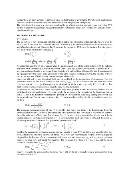
laminar flow are more difficult to represent since the RTD curve is asymmetric. Deviations of ideal laminar
flow are associated with coils or curves and also with tube roughness or corrugation.
The objective of this work is to propose generalized forms of the theoretical convective and power-law RTD
models in order to characterize non-ideal laminar flow in tubes and to test these models on a sanitary doublepipe
heat exchanger.
MATERIALS & METHODS
RTD Models
The theoretical E-curve associated with the parabolic radial velocity profile of laminar tube flow is given by
Eq. (2) that is known as the “convection model”. Variable is the mean residence time, which is calculated
as V/Q (volume/flow-rate). Likewise, Eq.(3) presents the theoretical RTD curve for the tube flow of a powerlaw
fluid, where n is the flow index [6, 7].
2
1
1
E t
t
(2)
3
2 t
2
n1
2n
2
n1
n 1
n 1
E t 1
3
3 1
3 1 t
(3)
n t n t
3n
1
Non-ideal laminar flow in tubes occurs when the relative roughness of the wall interferes with the velocity
profile or when the tube has curves or it is coiled. In this case, Eqs. (2) and (3) would fail to predict the RTD
and an experimental study is necessary. Large deviations from ideal flow with considerable dispersion could
be represented by the classic axial dispersion or the tanks-in-series models; however, the long tail of tracer
that is characteristic of laminar flow can not be captured correctly.
Since Eqs. (2) and (3) are theoretical, both can be modified by the introduction of parameters. The first
parameter would be the active volume of the vessel, V active , that is associated with the measured mean
residence time as V active = Q. Consequently, the dead volume of the vessel is given by V dead = V – V active . The
dead volume is related to undesirable stagnation and recirculation areas.
Adaptations of the convection model were previously used by other authors to describe laminar flow in
helical coils and chemical reactors [5]. In this work, the approach is the parameterize the breakthrough time
in Eq. (1) that is the minimum residence time given by ( = ½ for the ideal case). Taking into account that
the area under the E-curve must be unitary, Eq. (1) can be rewritten as Eq. (4), the “generalized convection
model”.
1
1
1
E t
t
(4)
1
t
t
The proposed parameterization of Eq. (3) is simpler: the power-law index n is disassociated from the
rheological behaviour of the liquid and turned into a free parameter. The flow index is related to the shape of
the radial velocity profile in tube flow through Eq. (5), where v b is the mean (bulk) velocity and R is the
internal radius of the tube. Note that for n = 1.0 the Newtonian parabolic profile is obtained. Equation (3)
with free parameter n constitutes the “generalized power-law model”.
n1
2
3n
1
r n
n1.
0
r
v r v 1
2v
1
(5)
b
b
n 1
R
R
Besides the generalized convection and power-law models, a third RTD model is also considered in this
work, which is the combined PFR+CSTR model. Its E-curve can easily model a long tail of tracer. Equation
(6) provides the E-curve of the combined model, where the parameters are plug and mix (mean residence
times of the plug flow and mixed flow regions). The mean residence time is = plug + mix and the active
volume is obtained from V active = Q [6, 7].
1 t
plug
E t exp
t
(6)
plug
mix
mix
Figure 1 presents the dimensionless E-curves (E = E) of the three models using a dimensionless time
variable that is = t/.