Generalized convection and power-law models to represent ... - USP

Generalized convection and power-law models to represent the residence time
distribution for non-ideal laminar flow in a double-pipe heat exchanger
Lucas K. Y. Murata , Jorge A. W. Gut
Department of Chemical Engineering, Escola Politécnica, University of São Paulo,
São Paulo, SP, Brazil (jorgewgut@usp.br)
ABSTRACT
The residence time distribution (RTD) is essential for the design and analysis of continuous thermal
processing equipment. For the processing of liquid foods, flow is usually laminar and the classic RTD models
often can not characterize non-ideal laminar flow. Such deviations are associated with coils, curves or tube
roughness/corrugation. Generalized forms of the theoretical convective and power-law models were proposed
in order to characterize non-ideal laminar flow in tubes. Introduced parameters were the breakthrough time
and the flow index, respectively. The combined PFR+CSTR model was also considered. To test the models,
experimental data was obtained from a sanitary double-pipe heat exchanger using an ionic tracer and a
conductivity flow cell. Tube diameter was 4.5 mm with a total length of 19.5 m and internal volume of 311
mL. Tested flow rates were between 12 and 20 L/h of distilled water (960 < Reynolds number < 1620). The
model E-curve was fitted to experimental data after numerical convolution with the E-curve of detection unit
to correct the signal distortion. Adjusted parameters were correlated with flow-rate. The best fit was obtained
with the combined model, followed by the generalized convection and generalized power-law models. The
adjusted flow index was under 1.0, suggesting that the velocity profile was flatter than the theoretical
parabola. This can be explained by the high roughness to diameter ratio of the tube. The higher breakthrough
time obtained from the convection model also indicates a flatter velocity profile. The combined model was
useful to determine the contribution of dead space and stagnation zones in the equipment, which are due to
the curves and thermocouple connections. The proposed models proved to be useful to represent RTD of
non-ideal laminar flow in a tubular system.
Keywords: residence time distribution; thermal processing; heat exchanger; laminar flow
INTRODUCTION
Many liquid food products, such dairy, fruit or egg products are subjected to continuous thermal processing
for inactivation of undesired microorganisms and enzymes that compromise the food safety and shelf-life.
Heat exchangers are used for rapidly heating and cooling the liquid stream, while a holding tube ensures the
desired holding time at the processing temperature. For the proper design and analysis of continuous thermal
processing equipment, the residence time and temperature distributions of the product inside the holding tube
and heat exchangers must be known. The association of these distributions provides the lethality for given
safety or quality attributes [1–5].
Characterization of the hydrodynamics of a vessel can be conducted by interpretation of its experimental
residence time distribution (RTD) data. The RTD of a vessel (single fluid, constant density, steady state) can
be determined by a stimulus response technique by which a tracer is introduced into the inlet stream and its
concentration C(t) is recorded at the outlet stream. This technique is widely used for the evaluation of
chemical reactors and packed beds. For an instantaneous pulse input signal, the age distribution function (Ecurve)
is obtained from Eq. (1), where C 0 is the tracer background concentration, if existent [6, 7].
C
t C0
E t
(1)
C
t C0
dt
0
For tube flow, the RTD is associated with the velocity profile and the turbulence. The ideal cases of parabolic
velocity profile (laminar flow) and flat velocity profile (plug flow) rarely describe the flow through real
systems. Since liquid foods often have moderate viscosities, flow is usually laminar with a considerable
radial velocity profile, which scatters the RTD. The departure from the idealized flow patterns can be
accounted for using RTD models to represent the experimental data. The well known RTD models of “axial
dispersion” or “tanks-in-series” can be used to describe non-ideal turbulent flow. Small deviations from

laminar flow are more difficult to represent since the RTD curve is asymmetric. Deviations of ideal laminar
flow are associated with coils or curves and also with tube roughness or corrugation.
The objective of this work is to propose generalized forms of the theoretical convective and power-law RTD
models in order to characterize non-ideal laminar flow in tubes and to test these models on a sanitary doublepipe
heat exchanger.
MATERIALS & METHODS
RTD Models
The theoretical E-curve associated with the parabolic radial velocity profile of laminar tube flow is given by
Eq. (2) that is known as the “convection model”. Variable is the mean residence time, which is calculated
as V/Q (volume/flow-rate). Likewise, Eq.(3) presents the theoretical RTD curve for the tube flow of a powerlaw
fluid, where n is the flow index [6, 7].
2
1
1
E t
t
(2)
3
2 t
2
n1
2n
2
n1
n 1
n 1
E t 1
3
3 1
3 1 t
(3)
n t n t
3n
1
Non-ideal laminar flow in tubes occurs when the relative roughness of the wall interferes with the velocity
profile or when the tube has curves or it is coiled. In this case, Eqs. (2) and (3) would fail to predict the RTD
and an experimental study is necessary. Large deviations from ideal flow with considerable dispersion could
be represented by the classic axial dispersion or the tanks-in-series models; however, the long tail of tracer
that is characteristic of laminar flow can not be captured correctly.
Since Eqs. (2) and (3) are theoretical, both can be modified by the introduction of parameters. The first
parameter would be the active volume of the vessel, V active , that is associated with the measured mean
residence time as V active = Q. Consequently, the dead volume of the vessel is given by V dead = V – V active . The
dead volume is related to undesirable stagnation and recirculation areas.
Adaptations of the convection model were previously used by other authors to describe laminar flow in
helical coils and chemical reactors [5]. In this work, the approach is the parameterize the breakthrough time
in Eq. (1) that is the minimum residence time given by ( = ½ for the ideal case). Taking into account that
the area under the E-curve must be unitary, Eq. (1) can be rewritten as Eq. (4), the “generalized convection
model”.
1
1
1
E t
t
(4)
1
t
t
The proposed parameterization of Eq. (3) is simpler: the power-law index n is disassociated from the
rheological behaviour of the liquid and turned into a free parameter. The flow index is related to the shape of
the radial velocity profile in tube flow through Eq. (5), where v b is the mean (bulk) velocity and R is the
internal radius of the tube. Note that for n = 1.0 the Newtonian parabolic profile is obtained. Equation (3)
with free parameter n constitutes the “generalized power-law model”.
n1
2
3n
1
r n
n1.
0
r
v r v 1
2v
1
(5)
b
b
n 1
R
R
Besides the generalized convection and power-law models, a third RTD model is also considered in this
work, which is the combined PFR+CSTR model. Its E-curve can easily model a long tail of tracer. Equation
(6) provides the E-curve of the combined model, where the parameters are plug and mix (mean residence
times of the plug flow and mixed flow regions). The mean residence time is = plug + mix and the active
volume is obtained from V active = Q [6, 7].
1 t
plug
E t exp
t
(6)
plug
mix
mix
Figure 1 presents the dimensionless E-curves (E = E) of the three models using a dimensionless time
variable that is = t/.

RTD Experiments
The RTD experiments were conducted on the heating section of a tubular continuous pasteurizer with
nominal capacity of 20 L/h (see Figure 2). The equipment was previously used for the pasteurization of
banana puree and mango puree. Tested fluid in this work was distilled water in laminar flow (flow-rate
between 12 and 20 L/h with Reynolds number between 960 and 1620). The heating section was a doublepipe
heat exchanger with five hairpins connected in series. The inner diameter was 4.5 mm and the total
length was 19.5 m (including the return bends). The internal volume was 311 mL.
12
12
10
0.1
0.9
a
10
0
b
8
0.2
0.8
8
n
0.3
0.1
E
6
0.3 0.7
E
6
0.6
4
0.4 0.6
0.5
4
2.0
1.0
2
2
E
0
0.0 0.5 1.0 1.5 2.0
12
10
8
6
4
2
0.9
plug
0.8
0.7
0.6
0.5
0.2 0.3 0.4
0.1
c
0
0.0 0.5 1.0 1.5 2.0
DTR Models:
a = generalized convection
b = generalized power-law
c = combined PFR+CSTR
0
0.0 0.5 1.0 1.5 2.0
Figure 1. Dimensionless E-curves for the RTD models considered in this work. Curves are from Eqs. (4), (3) and (6).
Figure 2. Photograph of the pasteurizer. Cooling heat exchanger at left and heating heat exchanger at right, with the
holding tube in between.
Sodium chloride was used as tracer, which was detected with a conductivity meter with flow-through cell
(YSI, Ohio, USA). Data acquisition frequency was 1 Hz. A low background concentration of NaCl was kept
to improve the strength of the conductivity signal. A small volume of saturated NaCl solution was injected
through a Tee at the entrance of the exchanger using a syringe. All experimental measurements were run in
quadruplicate. The tracer concentration was calculated from the electrical conductivity and temperature data
using a calibration equation [5]. The experimental values of E(t) were obtained through Eq. (1), using a
trapezoidal method to evaluate the integral.

Model adjustment
The RTD data from a pulse response experiment is affected by the way the tracer is injected and by how it is
detected. When measuring short residence times, the efficiency of the injection and detection units is of
considerable importance [8]. In order to take into account the signal distortion promoted by the detection
unit, its E-curve was determined for the same flow-rate and temperature conditions of the RTD experiments
and the model curve was convoluted with this E-curve before the model adjustment. The technique is
described in details elsewhere [5].
The two model parameters were adjusted in order to minimize the sum of squared errors of the convoluted
curve. The convolution was accomplished numerically in the time domain using a time step of 0.05, 0.10 or
0.20 s, depending on the time horizon. The number of discrete time points was 500. The Solver feature of
Excel (Microsoft, Redmond, USA), which uses a GRG2 algorithm, was applied to minimize the error
function after a good first estimate of the parameters was obtained by trial and error.
RESULTS & DISCUSSION
An example of E-curve fitting is presented in Figure 3 for a given experimental run. Each Et plot provides
the model curve, the convoluted curve and the experimental points. The clear difference between the model
curve and the convoluted curve shows that the signal distortion promoted by the detection unit is significant.
The experimental RTD data presented a long tail of tracer that is characteristic of laminar flow and/or
stagnation areas.
0.10
0.08
model
a
0.10
0.08
model
b
E (1/s)
0.06
0.04
convolution
E (1/s)
0.06
0.04
convolution
0.02
experimental
0.02
experimental
E (1/s)
0.00
0 20 40 60 80 100 120 140
t (s)
0.10
0.08
model
0.06
convolution
0.04
c
0.00
0 20 40 60 80 100 120 140
t (s)
DTR Models:
a = generalized convection
b = generalized power-law
0.02
experimental
c = combined PFR+CSTR
0.00
0 20 40 60 80 100 120 140
t (s)
Figure 3. Example of RTD model adjustment for a given experimental run (Q = 16.5 L/h). The sums of squared errors on
E were: a) 6.610 –4 , b) 14.110 –4 and c) 3.310 –4 .
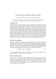
The model that provided the best fit for the considered flow-rate range was the combined PFR+CSTR model,
followed by the generalized convection model and by the generalized power-law model. The means of the
sum of squared errors on E were 4.410 –4 , 8.310 –4 and 14.510 –4 s –2 , respectively. The adjusted parameters
are presented in Figure 4.
According to Eq. (1), the theoretical breakthrough time for laminar flow is half of the mean residence time,
which corresponds to = 0.5. In Figure 4a it can be seen that > 0.5 was observed with a positive effect of
the flow rate. This deviation indicates the existence of secondary flow circulation that delayed the
breakthrough time for laminar flow in helical coils [9, 10]. Since the exchanger have ten return bends and
some tees for thermocouple connection, some internal recirculation may exist.
Figure 4b shows that the flow index for water was n < 1.0 that is characteristic of a pseudo-plastic fluid. The
velocity profile of a pseudoplastic fluid in laminar flow is flatter than the theoretical parabola for Newtonian

tube flow. The results indicate that the relative tube roughness altered the velocity profile by inducing some
turbulence near the wall, which consequently made the velocity profile flatter. The return bends and tees may
also have this effect locally. The negative effect of the flow-rate on n indicates a tendency towards plug-flow
with increasing flow rate.
1.0
1.1
0.9
0.8
y = 1.36E-02x + 4.27E-01
R 2 = 9.90E-01
1.0
0.9
theoretical n = 1.0
0.7
0.8
n
0.6
0.7
0.5
theoretical = 0.5
0.4
a
0.3
10 12 14 16 18 20 22
Q (L/h)
60
0.6
0.5
y = -2.55E-02x + 1.14E+00
R 2 = 8.18E-01
0.4
10 12 14 16 18 20 22
110
Q (L/h)
b
50
plug-flow
y = 7.08E+02x -1.03E+00
R 2 = 9.93E-01
100
90
40
80
convection
power-law
(s)
30
(s)
70
20
10
mixed-flow
y = 1.26E+03x -1.58E+00
R 2 = 9.92E-01
c
60
50
40
combined
theoretical
d
0
30
10 12 14 16 18 20 22
10 12 14 16 18 20 22
Q (L/h)
Q (L/h)
Figure 4. Summary of the results: a) parameter of the generalized convection model; b) parameter n of the generalized
power-law model; c) parameters plug and mix of the combined model (best fit in this work); d) mean residence time as
predicted by the three models and theory (V/Q).
0.09
E (1/s)
0.08
0.07
0.06
0.05
0.04
0.03
0.02
0.01
Theoretical
Gen. convection
Gen. Power-law
Combined (best fit)
0.00
0 20 40 60 80 100 120
Figure 5. Example of RTD model adjustment for a given experimental run (Q = 16.5 L/h). The sums of squared errors on
E were: a) 6.610 –4 , b) 14.110 –4 and c) 3.310 –4 .
t (s)

The best model fit was obtained with the combined PFR+CSTR model, whose parameters are presented in
Figure 4c. For laminar flow, parameter plug is actually the breakthrough time associated with the maximum
velocity at the centre of the tube. The difference between the convection and combined models resides on the
shape of the descending part or the curve. As can be noticed in Figure 2, the convection model better
represented this part of the curve.
The difference between the theoretical residence time and the residence time predicted by the combined
model can be seen in Figure 4d. This difference suggests that 19% of the internal volume of the exchanger is
associated with stagnation and recirculation regions.
Figure 5 brings the theoretical E-curve and the predictions from the adjusted RTD models for laminar flow in
the double-pipe heat exchanger with a flow rate of 15 L/h. It is clear that the proposed models could capture
the nonideality of the flow. The combined model provided the best fit, but the difference among the model
curves in Figure 5 is rather small. The curves in Figure 5 could be combined with the temperature
distribution along the exchanger in order to evaluate the distributed and integrated lethality in the heating
section of the exchanger [11].
CONCLUSIONS
The proposed models proved to be useful to represent RTD of non-laminar flow in tubular systems, which
are usually found in the continuous processing of liquid foods. The E-curve of these models can represent the
tail of tracer that is inherent in laminar flow. These models can be used in practice to represent the flow
patterns of tubular vessels and to diagnose deviations from non-ideal flow. Future testes will be conducted
using a glycerol/water mixture, which is a Newtonian viscous liquid, and a CMC solution, which is a pseudoplastic
viscous fluid.
ACKNOWLEDGMENTS
The authors wish to thank the São Paulo State Research Fund Agency (FAPESP 2009/07934-3) and the
National Council for Scientific and Technological Development (CNPq PIBIC) for financial support.
REFERENCES
[1] Toledo R.T. 1999. Fundamentals of Food Process Engineering. 2.ed. New York: Chapman & Hall.
[2] Lewis M. & Heppell N. 2000. Continuous Thermal Processing of Foods: Pasteurization and UHT Sterilization. Aspen
Publishers, Gaithersburg, USA.
[3] Torres A.P. & Oliveira F.A.R. 1998. Residence Time Distribution Studies in Continuous Thermal Processing of
Liquid Foods: a Review. Journal of Food Engineering, 36(1), 1–30.
[4] Torres A.P., Oliveira F.A.R. & Fortuna S.P. 1998. Residence Time Distribution of Liquids in a Continuous Tubular
Thermal Processing System - Part I: Relating RTD to Processing Conditions. Journal of Food Engineering, 35(2),
147–163.
[5] Gutierrez C.G.C.C., Dias E.F.T.S. & Gut J.A.W. 2010. Residence Time Distribution in Holding Tubes Using
Generalized Convection Model and Numerical Convolution for Non-Ideal Tracer Detection. Journal of Food
Engineering, 98, 248–256.
[6] Fogler H.S. 2005. Elements of Chemical Reaction Engineering. 4.ed. Prentice Hall, Upper Saddle River, USA.
[7] Levenspiel O. 1989. The Chemical Reactor Ominibook. Oregon State University, USA.
[8] Burton H. 1958. An Analysis of the Performance of an Ultra-High-Temperature Milk Sterilizing Plant: I. Introduction
and Physical Measurements. Journal of Dairy Research, 25(1), 75–84.
[9] Ruthven D.M. 1971. The Residence Time Distribution for Ideal Laminar Flow in a Helical Tube. Chemical
Engineering Science, 26, 1113–1121.
[10] Trivedi R.N. & Vasudeva K. 1974. RTD for Diffusion Free Laminar-Flow in Helical Coils. Chemical Engineering
Science, 29(12), 2291–2295.
[11] Rao M.A. & Loncin M. 1974. Residence Time Distribution and its Role in Continuous Pasteurization (Part II).
Lebensmittel-Wissenschaft und-Technologie, 7(1), 14–17.