Generalized convection and power-law models to represent ... - USP

Model adjustment
The RTD data from a pulse response experiment is affected by the way the tracer is injected and by how it is
detected. When measuring short residence times, the efficiency of the injection and detection units is of
considerable importance [8]. In order to take into account the signal distortion promoted by the detection
unit, its E-curve was determined for the same flow-rate and temperature conditions of the RTD experiments
and the model curve was convoluted with this E-curve before the model adjustment. The technique is
described in details elsewhere [5].
The two model parameters were adjusted in order to minimize the sum of squared errors of the convoluted
curve. The convolution was accomplished numerically in the time domain using a time step of 0.05, 0.10 or
0.20 s, depending on the time horizon. The number of discrete time points was 500. The Solver feature of
Excel (Microsoft, Redmond, USA), which uses a GRG2 algorithm, was applied to minimize the error
function after a good first estimate of the parameters was obtained by trial and error.
RESULTS & DISCUSSION
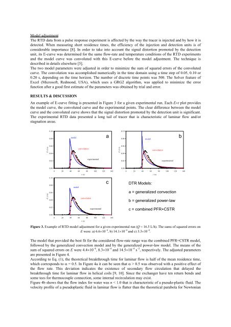
An example of E-curve fitting is presented in Figure 3 for a given experimental run. Each Et plot provides
the model curve, the convoluted curve and the experimental points. The clear difference between the model
curve and the convoluted curve shows that the signal distortion promoted by the detection unit is significant.
The experimental RTD data presented a long tail of tracer that is characteristic of laminar flow and/or
stagnation areas.
0.10
0.08
model
a
0.10
0.08
model
b
E (1/s)
0.06
0.04
convolution
E (1/s)
0.06
0.04
convolution
0.02
experimental
0.02
experimental
E (1/s)
0.00
0 20 40 60 80 100 120 140
t (s)
0.10
0.08
model
0.06
convolution
0.04
c
0.00
0 20 40 60 80 100 120 140
t (s)
DTR Models:
a = generalized convection
b = generalized power-law
0.02
experimental
c = combined PFR+CSTR
0.00
0 20 40 60 80 100 120 140
t (s)
Figure 3. Example of RTD model adjustment for a given experimental run (Q = 16.5 L/h). The sums of squared errors on
E were: a) 6.610 –4 , b) 14.110 –4 and c) 3.310 –4 .
The model that provided the best fit for the considered flow-rate range was the combined PFR+CSTR model,
followed by the generalized convection model and by the generalized power-law model. The means of the
sum of squared errors on E were 4.410 –4 , 8.310 –4 and 14.510 –4 s –2 , respectively. The adjusted parameters
are presented in Figure 4.
According to Eq. (1), the theoretical breakthrough time for laminar flow is half of the mean residence time,
which corresponds to = 0.5. In Figure 4a it can be seen that > 0.5 was observed with a positive effect of
the flow rate. This deviation indicates the existence of secondary flow circulation that delayed the
breakthrough time for laminar flow in helical coils [9, 10]. Since the exchanger have ten return bends and
some tees for thermocouple connection, some internal recirculation may exist.
Figure 4b shows that the flow index for water was n < 1.0 that is characteristic of a pseudo-plastic fluid. The
velocity profile of a pseudoplastic fluid in laminar flow is flatter than the theoretical parabola for Newtonian