Support Vector Machines - The Auton Lab
Support Vector Machines - The Auton Lab
Support Vector Machines - The Auton Lab

You also want an ePaper? Increase the reach of your titles
YUMPU automatically turns print PDFs into web optimized ePapers that Google loves.
<strong>Support</strong> <strong>Vector</strong><br />
<strong>Machines</strong><br />
Note to other teachers and users of<br />
these slides. Andrew would be delighted<br />
if you found this source material useful in<br />
giving your own lectures. Feel free to use<br />
these slides verbatim, or to modify them<br />
to fit your own needs. PowerPoint<br />
originals are available. If you make use<br />
of a significant portion of these slides in<br />
your own lecture, please include this<br />
message, or the following link to the<br />
source repository of Andrew’s tutorials:<br />
http://www.cs.cmu.edu/~awm/tutorials .<br />
Comments and corrections gratefully<br />
received.<br />
Andrew W. Moore<br />
Professor<br />
School of Computer Science<br />
Carnegie Mellon University<br />
www.cs.cmu.edu/~awm<br />
awm@cs.cmu.edu<br />
412-268-7599<br />
Copyright © 2001, 2003, Andrew W. Moore<br />
Nov 23rd, 2001<br />
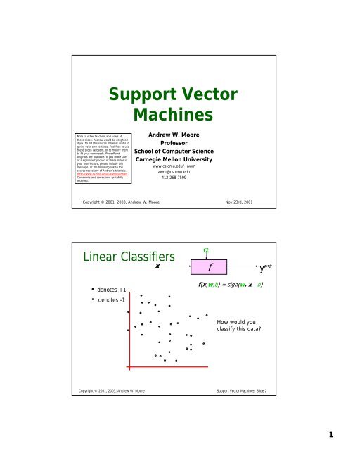
Linear Classifiers<br />
x<br />
α<br />
f<br />
y est<br />
denotes +1<br />
denotes -1<br />
f(x,w,b) = sign(w. x - b)<br />
How would you<br />
classify this data?<br />
Copyright © 2001, 2003, Andrew W. Moore <strong>Support</strong> <strong>Vector</strong> <strong>Machines</strong>: Slide 2<br />
1
Linear Classifiers<br />
x<br />
α<br />
f<br />
y est<br />
denotes +1<br />
denotes -1<br />
f(x,w,b) = sign(w. x - b)<br />
How would you<br />
classify this data?<br />
Copyright © 2001, 2003, Andrew W. Moore <strong>Support</strong> <strong>Vector</strong> <strong>Machines</strong>: Slide 3<br />
Linear Classifiers<br />
x<br />
α<br />
f<br />
y est<br />
denotes +1<br />
denotes -1<br />
f(x,w,b) = sign(w. x - b)<br />
How would you<br />
classify this data?<br />
Copyright © 2001, 2003, Andrew W. Moore <strong>Support</strong> <strong>Vector</strong> <strong>Machines</strong>: Slide 4<br />
2
Linear Classifiers<br />
x<br />
α<br />
f<br />
y est<br />
denotes +1<br />
denotes -1<br />
f(x,w,b) = sign(w. x - b)<br />
How would you<br />
classify this data?<br />
Copyright © 2001, 2003, Andrew W. Moore <strong>Support</strong> <strong>Vector</strong> <strong>Machines</strong>: Slide 5<br />
Linear Classifiers<br />
x<br />
α<br />
f<br />
y est<br />
denotes +1<br />
denotes -1<br />
f(x,w,b) = sign(w. x - b)<br />
Any of these<br />
would be fine..<br />
..but which is<br />
best?<br />
Copyright © 2001, 2003, Andrew W. Moore <strong>Support</strong> <strong>Vector</strong> <strong>Machines</strong>: Slide 6<br />
3
Classifier Margin<br />
x<br />
α<br />
f<br />
y est<br />
denotes +1<br />
denotes -1<br />
f(x,w,b) = sign(w. x - b)<br />
Define the margin<br />
of a linear<br />
classifier as the<br />
width that the<br />
boundary could be<br />
increased by<br />
before hitting a<br />
datapoint.<br />
Copyright © 2001, 2003, Andrew W. Moore <strong>Support</strong> <strong>Vector</strong> <strong>Machines</strong>: Slide 7<br />
Maximum Margin<br />
x<br />
α<br />
f<br />
y est<br />
denotes +1<br />
denotes -1<br />
Linear SVM<br />
f(x,w,b) = sign(w. x - b)<br />
<strong>The</strong> maximum<br />
margin linear<br />
classifier is the<br />
linear classifier<br />
with the, um,<br />
maximum margin.<br />
This is the<br />
simplest kind of<br />
SVM (Called an<br />
LSVM)<br />
Copyright © 2001, 2003, Andrew W. Moore <strong>Support</strong> <strong>Vector</strong> <strong>Machines</strong>: Slide 8<br />
4
Maximum Margin<br />
x<br />
α<br />
f<br />
y est<br />
denotes +1<br />
denotes -1<br />
<strong>Support</strong> <strong>Vector</strong>s<br />
are those<br />
datapoints that<br />
the margin<br />
pushes up<br />
against<br />
Linear SVM<br />
f(x,w,b) = sign(w. x - b)<br />
<strong>The</strong> maximum<br />
margin linear<br />
classifier is the<br />
linear classifier<br />
with the, um,<br />
maximum margin.<br />
This is the<br />
simplest kind of<br />
SVM (Called an<br />
LSVM)<br />
Copyright © 2001, 2003, Andrew W. Moore <strong>Support</strong> <strong>Vector</strong> <strong>Machines</strong>: Slide 9<br />
Why Maximum Margin?<br />
denotes +1<br />
denotes -1<br />
<strong>Support</strong> <strong>Vector</strong>s<br />
are those<br />
datapoints that<br />
the margin<br />
pushes up<br />
against<br />
1. Intuitively this feels safest.<br />
2. If we’ve made f(x,w,b) a small = sign(w. error in xthe<br />
- b)<br />
location of the boundary (it’s been<br />
jolted in its perpendicular <strong>The</strong> maximum direction)<br />
this gives us least margin chance linear of causing a<br />
misclassification. classifier is the<br />
3. LOOCV is easy since linear the classifier model is<br />
immune to removal with of the, any nonsupport-vector<br />
datapoints.<br />
um,<br />
maximum margin.<br />
4. <strong>The</strong>re’s some theory (using VC<br />
dimension) that is This related is the to (but not<br />
the same as) the simplest proposition kind that of this<br />
is a good thing. SVM (Called an<br />
5. Empirically it works LSVM) very very well.<br />
Copyright © 2001, 2003, Andrew W. Moore <strong>Support</strong> <strong>Vector</strong> <strong>Machines</strong>: Slide 10<br />
5
Specifying a line and margin<br />
“Predict Class = +1”<br />
zone<br />
“Predict Class = -1”<br />
zone<br />
Plus-Plane<br />
Classifier Boundary<br />
Minus-Plane<br />
• How do we represent this mathematically?<br />
• …in m input dimensions?<br />
Copyright © 2001, 2003, Andrew W. Moore <strong>Support</strong> <strong>Vector</strong> <strong>Machines</strong>: Slide 11<br />
Specifying a line and margin<br />
• Plus-plane = { x : w . x + b = +1 }<br />
• Minus-plane = { x : w . x + b = -1 }<br />
Classify as..<br />
“Predict Class = +1”<br />
zone<br />
wx+b=1<br />
wx+b=0<br />
wx+b=-1<br />
+1<br />
-1<br />
Universe<br />
explodes<br />
“Predict Class = -1”<br />
zone<br />
if<br />
if<br />
if<br />
Plus-Plane<br />
Classifier Boundary<br />
Minus-Plane<br />
w . x + b >= 1<br />
w . x + b
Computing the margin width<br />
“Predict Class = +1”<br />
zone<br />
wx+b=1<br />
wx+b=0<br />
wx+b=-1<br />
“Predict Class = -1”<br />
zone<br />
M = Margin Width<br />
How do we compute<br />
M in terms of w<br />
and b?<br />
• Plus-plane = { x : w . x + b = +1 }<br />
• Minus-plane = { x : w . x + b = -1 }<br />
Claim: <strong>The</strong> vector w is perpendicular to the Plus Plane. Why?<br />
Copyright © 2001, 2003, Andrew W. Moore <strong>Support</strong> <strong>Vector</strong> <strong>Machines</strong>: Slide 13<br />
Computing the margin width<br />
“Predict Class = +1”<br />
zone<br />
wx+b=1<br />
wx+b=0<br />
wx+b=-1<br />
“Predict Class = -1”<br />
zone<br />
• Plus-plane = { x : w . x + b = +1 }<br />
• Minus-plane = { x : w . x + b = -1 }<br />
Claim: <strong>The</strong> vector w is perpendicular to the Plus Plane. Why?<br />
And so of course the vector w is also<br />
perpendicular to the Minus Plane<br />
M = Margin Width<br />
How do we compute<br />
M in terms of w<br />
and b?<br />
Let u and v be two vectors on the<br />
Plus Plane. What is w . ( u – v ) ?<br />
Copyright © 2001, 2003, Andrew W. Moore <strong>Support</strong> <strong>Vector</strong> <strong>Machines</strong>: Slide 14<br />
7
Computing the margin width<br />
“Predict Class = +1”<br />
zone<br />
wx+b=1<br />
wx+b=0<br />
wx+b=-1<br />
“Predict Class = -1”<br />
zone<br />
M = Margin Width<br />
How do we compute<br />
M in terms of w<br />
and b?<br />
• Plus-plane = { x : w . x + b = +1 }<br />
• Minus-plane = { x : w . x + b = -1 }<br />
• <strong>The</strong> vector w is perpendicular to the Plus Plane<br />
• Let x - be any point on the minus plane<br />
• Let x + be the closest plus-plane-point to x - .<br />
x +<br />
x -<br />
Any location in<br />
R m : not<br />
necessarily a<br />
datapoint<br />
Copyright © 2001, 2003, Andrew W. Moore <strong>Support</strong> <strong>Vector</strong> <strong>Machines</strong>: Slide 15<br />
Computing the margin width<br />
“Predict Class = +1”<br />
zone<br />
wx+b=1<br />
wx+b=0<br />
wx+b=-1<br />
x +<br />
“Predict Class = -1”<br />
zone<br />
• Plus-plane = { x : w . x + b = +1 }<br />
• Minus-plane = { x : w . x + b = -1 }<br />
• <strong>The</strong> vector w is perpendicular to the Plus Plane<br />
• Let x - be any point on the minus plane<br />
• Let x + be the closest plus-plane-point to x - .<br />
• Claim: x + = x - + λ w for some value of λ. Why?<br />
x -<br />
M = Margin Width<br />
How do we compute<br />
M in terms of w<br />
and b?<br />
Copyright © 2001, 2003, Andrew W. Moore <strong>Support</strong> <strong>Vector</strong> <strong>Machines</strong>: Slide 16<br />
8
Computing the margin width<br />
<strong>The</strong> line from x - to x + is<br />
How perpendicular do we compute to the<br />
x -<br />
planes. M in terms of w<br />
So to and get b? from x - to x +<br />
travel some distance in<br />
• Plus-plane = { x : w . x + b = +1 direction } w.<br />
• Minus-plane = { x : w . x + b = -1 }<br />
• <strong>The</strong> vector w is perpendicular to the Plus Plane<br />
• Let x - be any point on the minus plane<br />
• Let x + be the closest plus-plane-point to x - .<br />
• Claim: x + = x - + λ w for some value of λ. Why?<br />
“Predict Class = +1”<br />
zone<br />
wx+b=1<br />
wx+b=0<br />
wx+b=-1<br />
x +<br />
“Predict Class = -1”<br />
zone<br />
M = Margin Width<br />
Copyright © 2001, 2003, Andrew W. Moore <strong>Support</strong> <strong>Vector</strong> <strong>Machines</strong>: Slide 17<br />
Computing the margin width<br />
What we know:<br />
• w . x + + b = +1<br />
• w . x - + b = -1<br />
• x + = x - + λ w<br />
• |x + - x - | = M<br />
It’s now easy to get M<br />
in terms of w and b<br />
“Predict Class = +1”<br />
zone<br />
wx+b=1<br />
wx+b=0<br />
wx+b=-1<br />
x +<br />
“Predict Class = -1”<br />
zone<br />
M = Margin Width<br />
Copyright © 2001, 2003, Andrew W. Moore <strong>Support</strong> <strong>Vector</strong> <strong>Machines</strong>: Slide 18<br />
x -<br />
9
Computing the margin width<br />
What we know:<br />
• w . x + + b = +1<br />
• w . x - + b = -1<br />
• x + = x - + λ w<br />
• |x + - x - | = M<br />
It’s now easy to get M<br />
in terms of w and b<br />
“Predict Class = +1”<br />
zone<br />
wx+b=1<br />
wx+b=0<br />
wx+b=-1<br />
x +<br />
“Predict Class = -1”<br />
zone<br />
M = Margin Width<br />
w . (x - + λ w) + b = 1<br />
=><br />
w . x - + b + λ w .w = 1<br />
=><br />
-1 + λ w .w = 1<br />
Copyright © 2001, 2003, Andrew W. Moore <strong>Support</strong> <strong>Vector</strong> <strong>Machines</strong>: Slide 19<br />
x -<br />
=><br />
λ =<br />
2<br />
w.w<br />
Computing the margin width<br />
What we know:<br />
• w . x + + b = +1<br />
• w . x - + b = -1<br />
• x + = x - + λ w<br />
• |x + - x - | = M<br />
• 2<br />
λ =<br />
w.w<br />
“Predict Class = +1”<br />
zone<br />
wx+b=1<br />
wx+b=0<br />
wx+b=-1<br />
x +<br />
“Predict Class = -1”<br />
zone<br />
M = Margin Width =<br />
M = |x + - x - | =| λ w |=<br />
Copyright © 2001, 2003, Andrew W. Moore <strong>Support</strong> <strong>Vector</strong> <strong>Machines</strong>: Slide 20<br />
x -<br />
= λ | w | = λ w.<br />
w<br />
2 w.<br />
w<br />
= =<br />
w.<br />
w<br />
2<br />
w.<br />
w<br />
2<br />
w.w<br />
10
Learning the Maximum Margin Classifier<br />
“Predict Class = +1”<br />
zone<br />
wx+b=1<br />
wx+b=0<br />
wx+b=-1<br />
“Predict Class = -1”<br />
zone<br />
Given a guess of w and b we can<br />
• Compute whether all data points in the correct half-planes<br />
• Compute the width of the margin<br />
So now we just need to write a program to search the space<br />
of w’s and b’s to find the widest margin that matches all<br />
the datapoints. How?<br />
Gradient descent? Simulated Annealing? Matrix Inversion?<br />
EM? Newton’s Method?<br />
x +<br />
M = Margin Width =<br />
Copyright © 2001, 2003, Andrew W. Moore <strong>Support</strong> <strong>Vector</strong> <strong>Machines</strong>: Slide 21<br />
x -<br />
2<br />
w. w<br />
Learning via Quadratic Programming<br />
• QP is a well-studied class of optimization<br />
algorithms to maximize a quadratic function of<br />
some real-valued variables subject to linear<br />
constraints.<br />
Copyright © 2001, 2003, Andrew W. Moore <strong>Support</strong> <strong>Vector</strong> <strong>Machines</strong>: Slide 22<br />
11
Find<br />
arg max<br />
u<br />
Quadratic Programming<br />
T<br />
T u Ru<br />
c + d u +<br />
2<br />
Quadratic criterion<br />
Subject to<br />
And subject to<br />
a<br />
a<br />
a<br />
a<br />
a<br />
a<br />
11<br />
21<br />
u + a<br />
u<br />
1<br />
1<br />
+ a<br />
u + a<br />
n1<br />
1<br />
( n+<br />
1)1<br />
( n+<br />
2)1<br />
( n+<br />
e)1<br />
u<br />
1<br />
1<br />
1<br />
12<br />
22<br />
n2<br />
u + a<br />
u + a<br />
+ a<br />
u<br />
u<br />
u<br />
2<br />
2<br />
2<br />
( n+<br />
1)2<br />
( n+<br />
2)2<br />
( n+<br />
e)2<br />
+ ... + a<br />
+ ... + a<br />
:<br />
+ ... + a<br />
u<br />
u<br />
u<br />
2<br />
2<br />
2<br />
:<br />
1m<br />
2m<br />
nm<br />
u<br />
u<br />
u<br />
m<br />
+ ... + a<br />
+ ... + a<br />
+ ... + a<br />
m<br />
m<br />
≤ b<br />
1<br />
≤ b<br />
2<br />
≤ b<br />
( n+<br />
1) m<br />
( n+<br />
e)<br />
m<br />
n<br />
( n+<br />
2) m<br />
u<br />
u<br />
u<br />
m<br />
m<br />
m<br />
= b<br />
= b<br />
= b<br />
n additional linear<br />
inequality<br />
constraints<br />
( n+<br />
1)<br />
( n+<br />
2)<br />
( n+<br />
e)<br />
e additional linear<br />
equality<br />
constraints<br />
Copyright © 2001, 2003, Andrew W. Moore <strong>Support</strong> <strong>Vector</strong> <strong>Machines</strong>: Slide 23<br />
Find<br />
arg max<br />
u<br />
Quadratic Programming<br />
T<br />
T u Ru<br />
c + d u +<br />
2<br />
Quadratic criterion<br />
Subject to<br />
And subject to<br />
a<br />
a<br />
a<br />
a<br />
a<br />
a<br />
11<br />
21<br />
u + a<br />
u<br />
1<br />
1<br />
+ a<br />
u + a<br />
n1<br />
1<br />
( n+<br />
1)1<br />
( n+<br />
2)1<br />
( n+<br />
e)1<br />
1<br />
1<br />
1<br />
12<br />
22<br />
n2<br />
u + a<br />
u + a<br />
u<br />
+ a<br />
u<br />
u<br />
u<br />
2<br />
2<br />
2<br />
( n+<br />
1)2<br />
( n+<br />
2)2<br />
( n+<br />
e)2<br />
+ ... + a<br />
+ ... + a<br />
:<br />
+ ... + a<br />
u<br />
u<br />
u<br />
2<br />
2<br />
2<br />
:<br />
1m<br />
2m<br />
nm<br />
u<br />
u<br />
u<br />
m<br />
+ ... + a<br />
+ ... + a<br />
+ ... + a<br />
m<br />
m<br />
≤ b<br />
1<br />
≤ b<br />
<strong>The</strong>re exist algorithms for finding<br />
such constrained quadratic<br />
optima much more efficiently<br />
and reliably than gradient<br />
ascent.<br />
2<br />
≤ b<br />
(But they are very fiddly…you<br />
probably don’t want to write<br />
one yourself)<br />
( n+<br />
1) m<br />
( n+<br />
e)<br />
m<br />
n<br />
( n+<br />
2) m<br />
u<br />
u<br />
u<br />
m<br />
m<br />
m<br />
= b<br />
= b<br />
= b<br />
n additional linear<br />
inequality<br />
constraints<br />
( n+<br />
1)<br />
( n+<br />
2)<br />
( n+<br />
e)<br />
e additional linear<br />
equality<br />
constraints<br />
Copyright © 2001, 2003, Andrew W. Moore <strong>Support</strong> <strong>Vector</strong> <strong>Machines</strong>: Slide 24<br />
12
Learning the Maximum Margin Classifier<br />
“Predict Class = +1”<br />
zone<br />
wx+b=1<br />
wx+b=0<br />
wx+b=-1<br />
“Predict Class = -1”<br />
zone<br />
M =<br />
2<br />
w.w<br />
Given guess of w , b we can<br />
• Compute whether all data<br />
points are in the correct<br />
half-planes<br />
• Compute the margin width<br />
Assume R datapoints, each<br />
(x k ,y k ) where y k = +/- 1<br />
What should our quadratic<br />
optimization criterion be?<br />
How many constraints will we<br />
have?<br />
What should they be?<br />
Copyright © 2001, 2003, Andrew W. Moore <strong>Support</strong> <strong>Vector</strong> <strong>Machines</strong>: Slide 25<br />
Learning the Maximum Margin Classifier<br />
“Predict Class = +1”<br />
zone<br />
wx+b=1<br />
wx+b=0<br />
wx+b=-1<br />
“Predict Class = -1”<br />
zone<br />
M =<br />
2<br />
w.w<br />
Given guess of w , b we can<br />
• Compute whether all data<br />
points are in the correct<br />
half-planes<br />
• Compute the margin width<br />
Assume R datapoints, each<br />
(x k ,y k ) where y k = +/- 1<br />
What should our quadratic<br />
optimization criterion be?<br />
Minimize w.w<br />
How many constraints will we<br />
have? R<br />
What should they be?<br />
w . x k + b >= 1 if y k = 1<br />
w . x k + b
Uh-oh!<br />
This is going to be a problem!<br />
What should we do?<br />
denotes +1<br />
denotes -1<br />
Copyright © 2001, 2003, Andrew W. Moore <strong>Support</strong> <strong>Vector</strong> <strong>Machines</strong>: Slide 27<br />
denotes +1<br />
denotes -1<br />
Uh-oh!<br />
This is going to be a problem!<br />
What should we do?<br />
Idea 1:<br />
Find minimum w.w, while<br />
minimizing number of<br />
training set errors.<br />
Problemette: Two things<br />
to minimize makes for<br />
an ill-defined<br />
optimization<br />
Copyright © 2001, 2003, Andrew W. Moore <strong>Support</strong> <strong>Vector</strong> <strong>Machines</strong>: Slide 28<br />
14
denotes +1<br />
denotes -1<br />
Uh-oh!<br />
This is going to be a problem!<br />
What should we do?<br />
Idea 1.1:<br />
Minimize<br />
w.w + C (#train errors)<br />
Tradeoff parameter<br />
<strong>The</strong>re’s a serious practical<br />
problem that’s about to make<br />
us reject this approach. Can<br />
you guess what it is?<br />
Copyright © 2001, 2003, Andrew W. Moore <strong>Support</strong> <strong>Vector</strong> <strong>Machines</strong>: Slide 29<br />
denotes +1<br />
denotes -1<br />
Uh-oh!<br />
This is going to be a problem!<br />
What should we do?<br />
Idea 1.1:<br />
Minimize<br />
w.w + C (#train errors)<br />
Tradeoff parameter<br />
Can’t be expressed as a Quadratic<br />
Programming problem.<br />
Solving it may be too slow.<br />
(Also, doesn’t distinguish between<br />
disastrous errors and near misses)<br />
<strong>The</strong>re’s a serious practical<br />
problem that’s about to make<br />
us reject this approach. Can<br />
you guess what it is?<br />
So… any<br />
other<br />
ideas?<br />
Copyright © 2001, 2003, Andrew W. Moore <strong>Support</strong> <strong>Vector</strong> <strong>Machines</strong>: Slide 30<br />
15
denotes +1<br />
denotes -1<br />
Uh-oh!<br />
This is going to be a problem!<br />
What should we do?<br />
Idea 2.0:<br />
Minimize<br />
w.w + C (distance of error<br />
points to their<br />
correct place)<br />
Copyright © 2001, 2003, Andrew W. Moore <strong>Support</strong> <strong>Vector</strong> <strong>Machines</strong>: Slide 31<br />
Learning Maximum Margin with Noise<br />
wx+b=1<br />
wx+b=0<br />
wx+b=-1<br />
M =<br />
2<br />
w.w<br />
Given guess of w , b we can<br />
• Compute sum of distances<br />
of points to their correct<br />
zones<br />
• Compute the margin width<br />
Assume R datapoints, each<br />
(x k ,y k ) where y k = +/- 1<br />
What should our quadratic<br />
optimization criterion be?<br />
How many constraints will we<br />
have?<br />
What should they be?<br />
Copyright © 2001, 2003, Andrew W. Moore <strong>Support</strong> <strong>Vector</strong> <strong>Machines</strong>: Slide 32<br />
16
Learning Maximum Margin with Noise<br />
wx+b=1<br />
wx+b=0<br />
wx+b=-1<br />
ε 2<br />
ε 11<br />
ε 7<br />
M =<br />
2<br />
w.w<br />
Given guess of w , b we can<br />
• Compute sum of distances<br />
of points to their correct<br />
zones<br />
• Compute the margin width<br />
Assume R datapoints, each<br />
(x k ,y k ) where y k = +/- 1<br />
What should our quadratic<br />
optimization criterion be?<br />
Minimize<br />
1<br />
2<br />
w.<br />
w + C<br />
R<br />
∑ ε k<br />
k = 1<br />
How many constraints will we<br />
have? R<br />
What should they be?<br />
w . x k + b >= 1-ε k if y k = 1<br />
w . x k + b = 1-ε k if y k = 1<br />
w . x k + b
Learning Maximum Margin with Noise<br />
wx+b=1<br />
wx+b=0<br />
wx+b=-1<br />
ε 2<br />
ε 11<br />
ε 7<br />
M =<br />
2<br />
w.w<br />
Given guess of w , b we can<br />
• Compute sum of distances<br />
of points to their correct<br />
zones<br />
• Compute the margin width<br />
Assume R datapoints, each<br />
(x k ,y k ) where y k = +/- 1<br />
What should our quadratic<br />
optimization criterion be?<br />
Minimize<br />
1<br />
2<br />
w.<br />
w + C<br />
R<br />
∑ ε k<br />
k = 1<br />
<strong>The</strong>re’s a bug in this QP. Can you spot it?<br />
How many constraints will we<br />
have? R<br />
What should they be?<br />
w . x k + b >= 1-ε k if y k = 1<br />
w . x k + b = 1-ε k if y k = 1<br />
w . x k + b = 0 for all k<br />
Copyright © 2001, 2003, Andrew W. Moore <strong>Support</strong> <strong>Vector</strong> <strong>Machines</strong>: Slide 36<br />
18
An Equivalent QP<br />
Maximize<br />
R<br />
∑<br />
α<br />
1<br />
−<br />
R<br />
R<br />
∑∑<br />
k<br />
k = 1 2 k = 1 l=<br />
1<br />
α α Q<br />
k<br />
l<br />
kl<br />
Warning: up until Rong Zhang spotted my error in<br />
Oct 2003, this equation had been wrong in earlier<br />
versions of the notes. This version is correct.<br />
where Q = y y x . x )<br />
kl<br />
k<br />
l<br />
(<br />
k l<br />
Subject to these<br />
constraints:<br />
0 ≤<br />
α k<br />
≤ C<br />
∀k<br />
R<br />
∑<br />
k = 1<br />
α k<br />
y k<br />
=<br />
0<br />
<strong>The</strong>n define:<br />
w =<br />
b<br />
R<br />
∑<br />
k = 1<br />
K<br />
α k<br />
y k<br />
x<br />
= y (1 − ε ) − x . w<br />
where K = arg max<br />
K<br />
k<br />
k<br />
K<br />
α<br />
K<br />
k<br />
<strong>The</strong>n classify with:<br />
f(x,w,b) = sign(w. x - b)<br />
Copyright © 2001, 2003, Andrew W. Moore <strong>Support</strong> <strong>Vector</strong> <strong>Machines</strong>: Slide 37<br />
An Equivalent QP<br />
R<br />
R R<br />
1<br />
∑αk<br />
− ∑∑αkαl<br />
Maximize where Q = y y x . x )<br />
k = 1 2 k = 1 l=<br />
1<br />
Q<br />
kl<br />
Warning: up until Rong Zhang spotted my error in<br />
Oct 2003, this equation had been wrong in earlier<br />
versions of the notes. This version is correct.<br />
kl<br />
k<br />
l<br />
(<br />
k l<br />
Subject to these<br />
constraints:<br />
0 ≤<br />
α k<br />
≤ C<br />
∀k<br />
R<br />
∑<br />
k = 1<br />
α k<br />
y k<br />
=<br />
0<br />
<strong>The</strong>n define:<br />
w<br />
=<br />
R<br />
∑<br />
k = 1<br />
α k<br />
y k<br />
x<br />
b = y<br />
K<br />
(1 − ε<br />
K<br />
) − x<br />
K<br />
. w<br />
where K = arg max α<br />
k<br />
k<br />
Datapoints with α k > 0<br />
will be the support<br />
vectors <strong>The</strong>n classify with:<br />
K<br />
k<br />
f(x,w,b) = sign(w. x - b)<br />
..so this sum only needs<br />
to be over the<br />
support vectors.<br />
Copyright © 2001, 2003, Andrew W. Moore <strong>Support</strong> <strong>Vector</strong> <strong>Machines</strong>: Slide 38<br />
19
R<br />
∑<br />
α<br />
An Equivalent QP<br />
1<br />
−<br />
R<br />
R<br />
∑∑<br />
k<br />
k = 1 2 k = 1 l=<br />
1<br />
α α Q<br />
Maximize where Q = y y x . x )<br />
k<br />
l<br />
Copyright © 2001, 2003, Andrew W. Moore <strong>Support</strong> <strong>Vector</strong> <strong>Machines</strong>: Slide 39<br />
kl<br />
kl<br />
k<br />
l<br />
(<br />
k l<br />
Why did I tell you about this R<br />
Subject to these equivalent 0 ≤ α k<br />
≤QP?<br />
C ∀k<br />
∑ α k<br />
y k<br />
constraints:<br />
• It’s a formulation that QP<br />
k = 1<br />
packages can optimize more<br />
<strong>The</strong>n define:<br />
quickly<br />
Datapoints with α k > 0<br />
will be the support<br />
R<br />
<strong>The</strong>n classify with:<br />
w = ∑ α k<br />
y<br />
•<br />
k<br />
xBecause of further vectors jawdropping<br />
developments<br />
k<br />
k = 1<br />
f(x,w,b) you’re = sign(w. x - b)<br />
about to learn. ..so this sum only needs<br />
b = y<br />
K<br />
(1 − ε<br />
K<br />
) − x<br />
K<br />
. w to be over the<br />
K<br />
support vectors.<br />
where<br />
K<br />
=<br />
arg<br />
max<br />
k<br />
α<br />
k<br />
=<br />
0<br />
Suppose we’re in 1-dimension<br />
What would<br />
SVMs do with<br />
this data?<br />
x=0<br />
Copyright © 2001, 2003, Andrew W. Moore <strong>Support</strong> <strong>Vector</strong> <strong>Machines</strong>: Slide 40<br />
20
Suppose we’re in 1-dimension<br />
Not a big surprise<br />
x=0<br />
Positive “plane”<br />
Negative “plane”<br />
Copyright © 2001, 2003, Andrew W. Moore <strong>Support</strong> <strong>Vector</strong> <strong>Machines</strong>: Slide 41<br />
Harder 1-dimensional dataset<br />
That’s wiped the<br />
smirk off SVM’s<br />
face.<br />
What can be<br />
done about<br />
this?<br />
x=0<br />
Copyright © 2001, 2003, Andrew W. Moore <strong>Support</strong> <strong>Vector</strong> <strong>Machines</strong>: Slide 42<br />
21
Harder 1-dimensional dataset<br />
Remember how<br />
permitting nonlinear<br />
basis<br />
functions made<br />
linear regression<br />
so much nicer?<br />
Let’s permit them<br />
here too<br />
2<br />
x=0<br />
z<br />
k<br />
= ( xk<br />
, xk<br />
)<br />
Copyright © 2001, 2003, Andrew W. Moore <strong>Support</strong> <strong>Vector</strong> <strong>Machines</strong>: Slide 43<br />
Harder 1-dimensional dataset<br />
Remember how<br />
permitting nonlinear<br />
basis<br />
functions made<br />
linear regression<br />
so much nicer?<br />
Let’s permit them<br />
here too<br />
2<br />
x=0<br />
z<br />
k<br />
= ( xk<br />
, xk<br />
)<br />
Copyright © 2001, 2003, Andrew W. Moore <strong>Support</strong> <strong>Vector</strong> <strong>Machines</strong>: Slide 44<br />
22
Common SVM basis functions<br />
z k = ( polynomial terms of x k of degree 1 to q )<br />
z k = ( radial basis functions of x k )<br />
⎛ | xk<br />
− c<br />
z<br />
k[<br />
j]<br />
= φ j<br />
( xk<br />
) = KernelFn<br />
⎜<br />
⎝ KW<br />
z k = ( sigmoid functions of x k )<br />
This is sensible.<br />
Is that the end of the story?<br />
No…there’s one more trick!<br />
j<br />
| ⎞<br />
⎟<br />
⎠<br />
Copyright © 2001, 2003, Andrew W. Moore <strong>Support</strong> <strong>Vector</strong> <strong>Machines</strong>: Slide 45<br />
⎛<br />
⎜<br />
⎜<br />
⎜<br />
⎜<br />
⎜<br />
⎜<br />
⎜<br />
⎜<br />
⎜<br />
⎜<br />
⎜<br />
⎜<br />
⎜<br />
Φ(x) =<br />
⎜<br />
⎜<br />
⎜<br />
⎜<br />
⎜<br />
⎜<br />
⎜<br />
⎜<br />
⎜<br />
⎜<br />
⎜<br />
⎜<br />
⎜<br />
⎝<br />
1<br />
2x<br />
2x<br />
2x<br />
2x<br />
m<br />
2<br />
1<br />
2<br />
2<br />
x<br />
x<br />
x<br />
:<br />
:<br />
2<br />
m<br />
2x<br />
x<br />
1<br />
2x<br />
x<br />
:<br />
1<br />
2x<br />
x<br />
1<br />
2x<br />
x<br />
m<br />
2x<br />
x<br />
:<br />
:<br />
2<br />
1<br />
1<br />
2<br />
2<br />
3<br />
3<br />
m<br />
x<br />
⎞<br />
⎟<br />
⎟<br />
⎟<br />
⎟<br />
⎟<br />
⎟<br />
⎟<br />
⎟<br />
⎟<br />
⎟<br />
⎟<br />
⎟<br />
⎟<br />
⎟<br />
⎟<br />
⎟<br />
⎟<br />
⎟<br />
⎟<br />
⎟<br />
⎟<br />
⎟<br />
⎟<br />
⎟<br />
⎟<br />
⎟<br />
⎠<br />
Constant Term<br />
Linear Terms<br />
Pure<br />
Quadratic<br />
Terms<br />
Quadratic<br />
Cross-Terms<br />
Quadratic<br />
Basis Functions<br />
Number of terms (assuming m input<br />
dimensions) = (m+2)-choose-2<br />
= (m+2)(m+1)/2<br />
= (as near as makes no difference) m 2 /2<br />
You may be wondering what those<br />
2 ’s are doing.<br />
•You should be happy that they do no<br />
harm<br />
•You’ll find out why they’re there<br />
soon.<br />
m−1<br />
m<br />
Copyright © 2001, 2003, Andrew W. Moore <strong>Support</strong> <strong>Vector</strong> <strong>Machines</strong>: Slide 46<br />
23
QP with basis functions<br />
Maximize<br />
R<br />
∑<br />
α<br />
1<br />
−<br />
R<br />
R<br />
∑∑<br />
k<br />
k = 1 2 k = 1 l=<br />
1<br />
α α Q<br />
k<br />
l<br />
Warning: up until Rong Zhang spotted my error in<br />
Oct 2003, this equation had been wrong in earlier<br />
versions of the notes. This version is correct.<br />
kl<br />
where Qkl<br />
= yk<br />
yl<br />
( Φ(<br />
xk<br />
). Φ(<br />
xl<br />
))<br />
Subject to these<br />
constraints:<br />
0 ≤<br />
α k<br />
≤ C<br />
∀k<br />
R<br />
∑<br />
k = 1<br />
α k<br />
y k<br />
=<br />
0<br />
<strong>The</strong>n define:<br />
w =<br />
b<br />
k s.t.<br />
= y (1 − ε ) − x . w<br />
K<br />
∑<br />
α k<br />
α<br />
y k k<br />
> 0<br />
where K = arg max<br />
K<br />
Φ ( x<br />
k<br />
K<br />
k<br />
)<br />
α<br />
K<br />
k<br />
<strong>The</strong>n classify with:<br />
f(x,w,b) = sign(w. φ(x) -b)<br />
Copyright © 2001, 2003, Andrew W. Moore <strong>Support</strong> <strong>Vector</strong> <strong>Machines</strong>: Slide 47<br />
Maximize<br />
Subject to these<br />
constraints:<br />
<strong>The</strong>n define:<br />
w<br />
=<br />
R<br />
∑<br />
k s.t.<br />
α<br />
∑<br />
QP with basis functions<br />
α k<br />
1<br />
−<br />
α<br />
y k k<br />
> 0<br />
0 ≤<br />
Φ ( x<br />
k<br />
α k<br />
b = y<br />
K<br />
(1 − ε<br />
K<br />
) − x<br />
K<br />
. w<br />
where K = arg max α<br />
R<br />
R<br />
∑∑<br />
k<br />
k = 1 2 k = 1 l=<br />
1<br />
α α Q<br />
k<br />
k<br />
l<br />
kl<br />
where Qkl<br />
= yk<br />
yl<br />
( Φ(<br />
xk<br />
). Φ(<br />
xl<br />
))<br />
≤ C<br />
)<br />
We must do R 2 /2 dot products to<br />
get this matrix ready. R<br />
K<br />
k<br />
∀k<br />
Each dot product requires m 2 /2<br />
additions and multiplications<br />
k = 1<br />
<strong>The</strong>n classify with: …or does it?<br />
f(x,w,b) = sign(w. φ(x) -b)<br />
Copyright © 2001, 2003, Andrew W. Moore <strong>Support</strong> <strong>Vector</strong> <strong>Machines</strong>: Slide 48<br />
∑<br />
α k<br />
y k<br />
<strong>The</strong> whole thing costs R 2 m 2 /4.<br />
Yeeks!<br />
=<br />
0<br />
24
Quadratic Dot<br />
Products<br />
⎛<br />
⎜<br />
⎜<br />
⎜<br />
⎜<br />
⎜<br />
⎜<br />
⎜<br />
⎜<br />
⎜<br />
⎜<br />
⎜<br />
⎜<br />
⎜<br />
Φ( a)<br />
• Φ(<br />
b)<br />
=<br />
⎜<br />
⎜<br />
⎜<br />
⎜<br />
⎜<br />
⎜<br />
⎜<br />
⎜<br />
⎜<br />
⎜<br />
⎜<br />
⎜<br />
⎜<br />
⎝<br />
a<br />
1<br />
2a<br />
2a<br />
2a<br />
:<br />
2a<br />
m<br />
2<br />
1<br />
2<br />
2<br />
a<br />
a<br />
:<br />
2<br />
m<br />
2a a<br />
1<br />
2a a<br />
:<br />
1<br />
2a a<br />
1<br />
2a a<br />
m<br />
2a<br />
a<br />
:<br />
:<br />
2<br />
1<br />
1<br />
2<br />
2<br />
3<br />
3<br />
m<br />
a<br />
⎞<br />
⎛<br />
⎟ ⎜<br />
⎟ ⎜ 2b1<br />
⎟ ⎜ 2b2<br />
⎟ ⎜<br />
⎟ ⎜ :<br />
⎟ ⎜<br />
⎟ ⎜<br />
2bm<br />
2<br />
⎟ ⎜ b1<br />
⎟ ⎜ 2<br />
⎟ ⎜ b2<br />
⎟ ⎜ :<br />
⎟ ⎜<br />
2<br />
⎟ ⎜ bm<br />
⎟<br />
•<br />
⎜ 2b1b<br />
2<br />
⎟<br />
2b b<br />
⎟<br />
⎟<br />
⎟<br />
⎟<br />
⎟<br />
⎟<br />
⎟<br />
⎟<br />
⎟<br />
⎟<br />
⎟<br />
⎠<br />
⎜<br />
⎜<br />
⎜<br />
⎜<br />
⎜<br />
⎜<br />
⎜<br />
⎜<br />
⎜<br />
⎜<br />
⎜<br />
⎜<br />
⎝<br />
1<br />
:<br />
2b b<br />
2b<br />
1 3<br />
1 m<br />
2b<br />
b<br />
:<br />
2 3<br />
2b b<br />
1 m<br />
:<br />
b<br />
⎞<br />
⎟<br />
⎟<br />
⎟<br />
⎟<br />
⎟<br />
⎟<br />
⎟<br />
⎟<br />
⎟<br />
⎟<br />
⎟<br />
⎟<br />
⎟<br />
⎟<br />
⎟<br />
⎟<br />
⎟<br />
⎟<br />
⎟<br />
⎟<br />
⎟<br />
⎟<br />
⎟<br />
⎟<br />
⎟<br />
⎟<br />
⎠<br />
m−1<br />
m<br />
m−1<br />
m<br />
Copyright © 2001, 2003, Andrew W. Moore <strong>Support</strong> <strong>Vector</strong> <strong>Machines</strong>: Slide 49<br />
1<br />
+<br />
m<br />
∑<br />
i=<br />
1<br />
+<br />
m<br />
∑<br />
i=<br />
1<br />
m<br />
+<br />
2 a b i i<br />
a 2<br />
b i i<br />
m<br />
∑∑<br />
i= 1 j=<br />
i+<br />
1<br />
2<br />
2a a b b<br />
i<br />
j<br />
i<br />
j<br />
Quadratic Dot<br />
Products<br />
Φ( a)<br />
• Φ(<br />
b)<br />
=<br />
1+<br />
2<br />
m<br />
∑<br />
i=<br />
1<br />
a b +<br />
i<br />
i<br />
m<br />
∑<br />
i=<br />
1<br />
a b<br />
2 2<br />
i i<br />
+<br />
m<br />
m<br />
∑∑<br />
i= 1 j=<br />
i+<br />
1<br />
2a a b b<br />
i<br />
j<br />
i<br />
j<br />
Just out of casual, innocent, interest,<br />
let’s look at another function of a and<br />
b:<br />
( a.<br />
b + 1)<br />
2<br />
= ( a.<br />
b)<br />
+ 2a.<br />
b + 1<br />
2<br />
2<br />
m<br />
m<br />
⎛ ⎞<br />
= ⎜∑<br />
aibi<br />
⎟ + 2∑<br />
aibi<br />
+ 1<br />
⎝ i=<br />
1 ⎠ i=<br />
1<br />
m<br />
m<br />
= ∑∑aibia<br />
jb<br />
j<br />
+ 2∑<br />
aibi<br />
+ 1<br />
i= 1 j=<br />
1<br />
m<br />
m<br />
i=<br />
1<br />
= 2<br />
∑ ( a ) + 2∑∑<br />
+ 2 ∑<br />
ibi<br />
aibi<br />
a<br />
jb<br />
j<br />
aibi<br />
+ 1<br />
i=<br />
1<br />
m<br />
m<br />
i= 1 j=<br />
i+<br />
1<br />
m<br />
i=<br />
1<br />
Copyright © 2001, 2003, Andrew W. Moore <strong>Support</strong> <strong>Vector</strong> <strong>Machines</strong>: Slide 50<br />
25
Quadratic Dot<br />
Products<br />
Φ( a)<br />
• Φ(<br />
b)<br />
=<br />
1+<br />
2<br />
m<br />
∑<br />
i=<br />
1<br />
a b +<br />
i<br />
i<br />
m<br />
∑<br />
i=<br />
1<br />
a b<br />
2 2<br />
i i<br />
+<br />
m<br />
m<br />
∑∑<br />
i= 1 j=<br />
i+<br />
1<br />
2a a b b<br />
i<br />
j<br />
i<br />
j<br />
Just out of casual, innocent, interest,<br />
let’s look at another function of a and<br />
b:<br />
( a.<br />
b + 1)<br />
2<br />
= ( a.<br />
b)<br />
+ 2a.<br />
b + 1<br />
2<br />
2<br />
m<br />
m<br />
⎛ ⎞<br />
= ⎜∑<br />
aibi<br />
⎟ + 2∑<br />
aibi<br />
+ 1<br />
⎝ i=<br />
1 ⎠ i=<br />
1<br />
m<br />
m<br />
= ∑∑aibia<br />
jb<br />
j<br />
+ 2∑<br />
aibi<br />
+ 1<br />
i= 1 j=<br />
1<br />
m<br />
m<br />
i=<br />
1<br />
= 2<br />
∑ ( a ) + 2∑∑<br />
+ 2 ∑<br />
ibi<br />
aibi<br />
a<br />
jb<br />
j<br />
aibi<br />
+ 1<br />
i=<br />
1<br />
m<br />
m<br />
i= 1 j=<br />
i+<br />
1<br />
m<br />
i=<br />
1<br />
<strong>The</strong>y’re the same!<br />
And this is only O(m) to<br />
compute!<br />
Copyright © 2001, 2003, Andrew W. Moore <strong>Support</strong> <strong>Vector</strong> <strong>Machines</strong>: Slide 51<br />
Maximize<br />
QP with Quadratic basis functions<br />
R<br />
R R<br />
1<br />
∑αk<br />
− ∑∑αkαlQkl<br />
Qkl<br />
= yk<br />
yl<br />
Φ(<br />
xk<br />
).<br />
k = 1 2 k = 1 l=<br />
1<br />
Subject to these<br />
constraints:<br />
0 ≤<br />
α k<br />
≤ C<br />
where ( Φ(<br />
xl<br />
))<br />
We must do R 2 /2 dot products to<br />
get this matrix ready. R<br />
∀k<br />
Warning: up until Rong Zhang spotted my error in<br />
Oct 2003, this equation had been wrong in earlier<br />
versions of the notes. This version is correct.<br />
∑<br />
α k<br />
y k<br />
Each dot product now only requires<br />
m additions and multiplications<br />
k = 1<br />
=<br />
0<br />
<strong>The</strong>n define:<br />
w =<br />
b<br />
k s.t.<br />
= y (1 − ε ) − x . w<br />
K<br />
∑<br />
α k<br />
α<br />
y k k<br />
> 0<br />
where K = arg max<br />
K<br />
Φ ( x<br />
k<br />
K<br />
k<br />
)<br />
α<br />
K<br />
k<br />
<strong>The</strong>n classify with:<br />
f(x,w,b) = sign(w. φ(x) -b)<br />
Copyright © 2001, 2003, Andrew W. Moore <strong>Support</strong> <strong>Vector</strong> <strong>Machines</strong>: Slide 52<br />
26
Higher Order Polynomials<br />
Polynomial<br />
Quadratic<br />
Cubic<br />
Quartic<br />
φ(x)<br />
All m 2 /2<br />
terms up to<br />
degree 2<br />
All m 3 /6<br />
terms up to<br />
degree 3<br />
All m 4 /24<br />
terms up to<br />
degree 4<br />
Cost to<br />
build Q kl<br />
matrix<br />
tradition<br />
ally<br />
m 2 R 2 /4<br />
Cost if 100<br />
inputs<br />
2,500 R 2<br />
m 3 R 2 /12 83,000 R 2<br />
m 4 R 2 /48 1,960,000 R 2<br />
Cost to<br />
build Q kl<br />
matrix<br />
sneakily<br />
φ(a).φ(b)<br />
(a.b+1) 2<br />
(a.b+1) 3<br />
(a.b+1) 4<br />
mR 2 / 2<br />
mR 2 / 2<br />
mR 2 / 2<br />
Cost if<br />
100<br />
inputs<br />
50 R 2<br />
50 R 2<br />
50 R 2<br />
Copyright © 2001, 2003, Andrew W. Moore <strong>Support</strong> <strong>Vector</strong> <strong>Machines</strong>: Slide 53<br />
QP with Quintic basis functions<br />
We must do R 2 /2 dot products R R to get this<br />
matrix ready.<br />
Maximize ∑αk<br />
+ ∑∑αkαlQ<br />
where Q ( ( ). ( ))<br />
kl<br />
kl<br />
= yk<br />
yl<br />
Φ xk<br />
Φ xl<br />
In 100-d, each k = 1dot product k = 1now l=<br />
1 needs 103<br />
operations instead of 75 million<br />
R<br />
But there are still worrying things lurking away.<br />
Subject to these<br />
What are they? 0 ≤ α k<br />
≤ C ∀k<br />
∑ α k<br />
y k<br />
= 0<br />
constraints:<br />
k = 1<br />
<strong>The</strong>n define:<br />
w =<br />
b<br />
k s.t.<br />
K<br />
∑<br />
α k<br />
α<br />
y k k<br />
> 0<br />
K<br />
Φ ( x<br />
= y (1 − ε ) − x . w<br />
where K = arg max<br />
k<br />
K<br />
k<br />
)<br />
α<br />
K<br />
k<br />
<strong>The</strong>n classify with:<br />
f(x,w,b) = sign(w. φ(x) -b)<br />
Copyright © 2001, 2003, Andrew W. Moore <strong>Support</strong> <strong>Vector</strong> <strong>Machines</strong>: Slide 54<br />
27
Maximize<br />
QP with Quintic basis functions<br />
We must do R 2 /2 dot products R R to get this<br />
matrix ready.<br />
∑αk<br />
+ ∑∑αkαlQ<br />
where Q ( ( ). ( ))<br />
kl<br />
kl<br />
= yk<br />
yl<br />
Φ xk<br />
Φ xl<br />
In 100-d, each k = 1dot product k = 1now l=<br />
1 needs 103<br />
operations instead of 75 million<br />
R<br />
But there are still worrying things lurking away.<br />
Subject to these<br />
What are they? 0 ≤ α k<br />
≤ C ∀k<br />
∑ α k<br />
y k<br />
= 0<br />
constraints:<br />
•<strong>The</strong> fear of overfitting kwith = 1 this enormous<br />
number of terms<br />
<strong>The</strong>n define:<br />
•<strong>The</strong> evaluation phase (doing a set of<br />
predictions on a test set) will be very<br />
expensive (why?)<br />
w<br />
=<br />
k s.t.<br />
∑<br />
α k<br />
α<br />
y k k<br />
> 0<br />
Φ ( x<br />
b = y<br />
K<br />
(1 − ε<br />
K<br />
) − x<br />
K<br />
. w<br />
where K = arg max α<br />
k<br />
k<br />
)<br />
K<br />
k<br />
<strong>The</strong>n classify with:<br />
f(x,w,b) = sign(w. φ(x) -b)<br />
Copyright © 2001, 2003, Andrew W. Moore <strong>Support</strong> <strong>Vector</strong> <strong>Machines</strong>: Slide 55<br />
Maximize<br />
QP with Quintic basis functions<br />
We must do R 2 /2 dot products R R to get this<br />
matrix ready.<br />
∑αk<br />
+ ∑∑αkαlQ<br />
where Q ( ( ). ( ))<br />
kl<br />
kl<br />
= yk<br />
yl<br />
Φ xk<br />
Φ xl<br />
In 100-d, each k = 1dot product k = 1now l=<br />
1 needs 103<br />
<strong>The</strong> use of Maximum Margin<br />
operations instead of 75 million<br />
magically makes this not a<br />
problem R<br />
But there are still worrying things lurking away.<br />
Subject to these<br />
What are they? 0 ≤ α k<br />
≤ C ∀k<br />
∑ α k<br />
y k<br />
= 0<br />
constraints:<br />
•<strong>The</strong> fear of overfitting kwith = 1 this enormous<br />
number of terms<br />
<strong>The</strong>n define:<br />
•<strong>The</strong> evaluation phase (doing a set of<br />
predictions on a test set) will be very<br />
expensive (why?)<br />
w<br />
=<br />
k s.t.<br />
∑<br />
α k<br />
α<br />
y k k<br />
> 0<br />
Φ ( x<br />
b = y<br />
K<br />
(1 − ε<br />
K<br />
) − x<br />
K<br />
. w<br />
where K = arg max α<br />
k<br />
k<br />
)<br />
K<br />
k<br />
Because each w. φ(x) (see below)<br />
needs 75 million operations. What<br />
can be done?<br />
<strong>The</strong>n classify with:<br />
f(x,w,b) = sign(w. φ(x) -b)<br />
Copyright © 2001, 2003, Andrew W. Moore <strong>Support</strong> <strong>Vector</strong> <strong>Machines</strong>: Slide 56<br />
28
Maximize<br />
QP with Quintic basis functions<br />
We must do R 2 /2 dot products R R to get this<br />
matrix ready.<br />
∑αk<br />
+ ∑∑αkαlQ<br />
where Q ( ( ). ( ))<br />
kl<br />
kl<br />
= yk<br />
yl<br />
Φ xk<br />
Φ xl<br />
In 100-d, each k = 1dot product k = 1now l=<br />
1 needs 103<br />
<strong>The</strong> use of Maximum Margin<br />
operations instead of 75 million<br />
magically makes this not a<br />
problem R<br />
But there are still worrying things lurking away.<br />
Subject to these<br />
What are they? 0 ≤ α k<br />
≤ C ∀k<br />
∑ α k<br />
y k<br />
= 0<br />
constraints:<br />
•<strong>The</strong> fear of overfitting kwith = 1 this enormous<br />
number of terms<br />
<strong>The</strong>n define:<br />
•<strong>The</strong> evaluation phase (doing a set of<br />
predictions on a test set) will be very<br />
expensive (why?)<br />
w<br />
=<br />
k s.t.<br />
∑<br />
α k<br />
α<br />
y k k<br />
> 0<br />
Φ ( x<br />
wb<br />
⋅= Φ ( yx<br />
) =<br />
K<br />
(1 −∑<br />
εα<br />
k<br />
y<br />
K<br />
) k<br />
Φ−<br />
(<br />
x<br />
k<br />
)<br />
K<br />
. ⋅wΦ<br />
k s.t. α k > 0<br />
where<br />
=<br />
K∑=<br />
α<br />
arg k<br />
y k<br />
( xmax<br />
k<br />
⋅ x + 1)<br />
α<br />
k s.t. α k > 0<br />
k<br />
k<br />
Only Sm operations (S=#support vectors)<br />
k<br />
)<br />
( x )<br />
K<br />
5<br />
Because each w. φ(x) (see below)<br />
needs 75 million operations. What<br />
can be done?<br />
<strong>The</strong>n classify with:<br />
f(x,w,b) = sign(w. φ(x) -b)<br />
Copyright © 2001, 2003, Andrew W. Moore <strong>Support</strong> <strong>Vector</strong> <strong>Machines</strong>: Slide 57<br />
Maximize<br />
QP with Quintic basis functions<br />
We must do R 2 /2 dot products R R to get this<br />
matrix ready.<br />
∑αk<br />
+ ∑∑αkαlQ<br />
where Q ( ( ). ( ))<br />
kl<br />
kl<br />
= yk<br />
yl<br />
Φ xk<br />
Φ xl<br />
In 100-d, each k = 1dot product k = 1now l=<br />
1 needs 103<br />
<strong>The</strong> use of Maximum Margin<br />
operations instead of 75 million<br />
magically makes this not a<br />
problem R<br />
But there are still worrying things lurking away.<br />
Subject to these<br />
What are they? 0 ≤ α k<br />
≤ C ∀k<br />
∑ α k<br />
y k<br />
= 0<br />
constraints:<br />
•<strong>The</strong> fear of overfitting kwith = 1 this enormous<br />
number of terms<br />
<strong>The</strong>n define:<br />
•<strong>The</strong> evaluation phase (doing a set of<br />
predictions on a test set) will be very<br />
expensive (why?)<br />
wb<br />
w<br />
⋅<br />
=<br />
k s.t.<br />
∑<br />
α k<br />
α<br />
y k k<br />
> 0<br />
Φ ( x<br />
= Φ ( yx<br />
) = (1 −∑<br />
εα<br />
) Φ−<br />
(<br />
x ) . ⋅wΦ<br />
k<br />
)<br />
Because each w. φ(x) (see below)<br />
needs 75 million operations. What<br />
can be done?<br />
k<br />
y k k<br />
K k s.t. α k > 0K<br />
K K<br />
5 <strong>The</strong>n When classify you see this with: many callout bubbles on<br />
where<br />
=<br />
K∑=<br />
α<br />
arg k<br />
y k<br />
( xmax<br />
k<br />
⋅ x + 1)<br />
α<br />
a slide it’s time to wrap the author in a<br />
k s.t. α k > 0<br />
k<br />
blanket, gently take him away and murmur<br />
k<br />
f(x,w,b) “someone’s = been sign(w. at the PowerPoint φ(x) -b) for too<br />
long.”<br />
Copyright © 2001, 2003, Andrew W. Moore <strong>Support</strong> <strong>Vector</strong> <strong>Machines</strong>: Slide 58<br />
Only Sm operations (S=#support vectors)<br />
( x )<br />
29
QP with Quintic basis functions<br />
1<br />
R<br />
R R<br />
Maximize ∑αk<br />
− ∑∑αkαlQkl<br />
where Andrew’s Qkl<br />
= opinion yk<br />
yl<br />
of ( Φwhy ( xSVMs k<br />
). Φdon’t<br />
( xl<br />
))<br />
k = 1 2 k = 1 l=<br />
1<br />
overfit as much as you’d think:<br />
No matter what the basis function,<br />
there are really Ronly up to R<br />
Subject to these 0 ≤ α k<br />
≤ C parameters: ∀k<br />
α∑<br />
1 , α 2 .. αα kR , yand k<br />
usually = 0<br />
constraints:<br />
most are set to<br />
k<br />
zero<br />
= 1<br />
by the Maximum<br />
Margin.<br />
<strong>The</strong>n define:<br />
Asking for small w.w is like “weight<br />
decay” in Neural Nets and like Ridge<br />
w = ∑ α y Φ k k<br />
( x<br />
Regression parameters in Linear<br />
k<br />
) regression and like the use of Priors<br />
in Bayesian Regression---all designed<br />
k s.t. α k > 0<br />
to smooth the function and reduce<br />
wb<br />
⋅= Φ (<br />
overfitting.<br />
yx<br />
) =<br />
K<br />
(1 −∑<br />
εα<br />
k<br />
y<br />
K<br />
) k<br />
Φ−<br />
(<br />
x<br />
k<br />
)<br />
K<br />
. ⋅wΦ<br />
( x )<br />
k s.t. α k > 0<br />
K<br />
5 <strong>The</strong>n classify with:<br />
where<br />
=<br />
K∑=<br />
α<br />
arg k<br />
y k<br />
( xmax<br />
k<br />
⋅ x + 1)<br />
α<br />
k s.t. α k > 0<br />
k<br />
k<br />
Only Sm operations (S=#support vectors) f(x,w,b) = sign(w. φ(x) -b)<br />
Copyright © 2001, 2003, Andrew W. Moore <strong>Support</strong> <strong>Vector</strong> <strong>Machines</strong>: Slide 59<br />
SVM Kernel Functions<br />
• K(a,b)=(a . b +1) d is an example of an SVM<br />
Kernel Function<br />
• Beyond polynomials there are other very high<br />
dimensional basis functions that can be made<br />
practical by finding the right Kernel Function<br />
• Radial-Basis-style Kernel Function:<br />
K(<br />
a,<br />
b)<br />
⎛ ( a − b)<br />
exp<br />
⎜−<br />
⎝ 2σ<br />
=<br />
2<br />
• Neural-net-style Kernel Function:<br />
K( a,<br />
b)<br />
= tanh( κ a.<br />
b −δ<br />
)<br />
2<br />
⎞<br />
⎟<br />
⎠<br />
σ, κ and δ are magic<br />
parameters that must<br />
be chosen by a model<br />
selection method<br />
such as CV or<br />
VCSRM*<br />
*see last lecture<br />
Copyright © 2001, 2003, Andrew W. Moore <strong>Support</strong> <strong>Vector</strong> <strong>Machines</strong>: Slide 60<br />
30
VC-dimension of an SVM<br />
• Very very very loosely speaking there is some theory which<br />
under some different assumptions puts an upper bound on<br />
the VC dimension as<br />
⎡<br />
⎢<br />
Diameter<br />
Margin<br />
• where<br />
• Diameter is the diameter of the smallest sphere that can<br />
enclose all the high-dimensional term-vectors derived<br />
from the training set.<br />
• Margin is the smallest margin we’ll let the SVM use<br />
• This can be used in SRM (Structural Risk Minimization) for<br />
choosing the polynomial degree, RBF σ, etc.<br />
• But most people just use Cross-Validation<br />
⎤<br />
⎥<br />
Copyright © 2001, 2003, Andrew W. Moore <strong>Support</strong> <strong>Vector</strong> <strong>Machines</strong>: Slide 61<br />
SVM Performance<br />
• Anecdotally they work very very well indeed.<br />
• Example: <strong>The</strong>y are currently the best-known<br />
classifier on a well-studied hand-written-character<br />
recognition benchmark<br />
• Another Example: Andrew knows several reliable<br />
people doing practical real-world work who claim<br />
that SVMs have saved them when their other<br />
favorite classifiers did poorly.<br />
• <strong>The</strong>re is a lot of excitement and religious fervor<br />
about SVMs as of 2001.<br />
• Despite this, some practitioners (including your<br />
lecturer) are a little skeptical.<br />
Copyright © 2001, 2003, Andrew W. Moore <strong>Support</strong> <strong>Vector</strong> <strong>Machines</strong>: Slide 62<br />
31
Doing multi-class classification<br />
• SVMs can only handle two-class outputs (i.e. a<br />
categorical output variable with arity 2).<br />
• What can be done?<br />
• Answer: with output arity N, learn N SVM’s<br />
• SVM 1 learns “Output==1” vs “Output != 1”<br />
• SVM 2 learns “Output==2” vs “Output != 2”<br />
• :<br />
• SVM N learns “Output==N” vs “Output != N”<br />
• <strong>The</strong>n to predict the output for a new input, just<br />
predict with each SVM and find out which one puts<br />
the prediction the furthest into the positive region.<br />
Copyright © 2001, 2003, Andrew W. Moore <strong>Support</strong> <strong>Vector</strong> <strong>Machines</strong>: Slide 63<br />
References<br />
• An excellent tutorial on VC-dimension and <strong>Support</strong><br />
<strong>Vector</strong> <strong>Machines</strong>:<br />
C.J.C. Burges. A tutorial on support vector machines<br />
for pattern recognition. Data Mining and Knowledge<br />
Discovery, 2(2):955-974, 1998.<br />
http://citeseer.nj.nec.com/burges98tutorial.html<br />
• <strong>The</strong> VC/SRM/SVM Bible:<br />
Statistical Learning <strong>The</strong>ory by Vladimir Vapnik, Wiley-<br />
Interscience; 1998<br />
Copyright © 2001, 2003, Andrew W. Moore <strong>Support</strong> <strong>Vector</strong> <strong>Machines</strong>: Slide 64<br />
32
What You Should Know<br />
• Linear SVMs<br />
• <strong>The</strong> definition of a maximum margin classifier<br />
• What QP can do for you (but, for this class, you<br />
don’t need to know how it does it)<br />
• How Maximum Margin can be turned into a QP<br />
problem<br />
• How we deal with noisy (non-separable) data<br />
• How we permit non-linear boundaries<br />
• How SVM Kernel functions permit us to pretend<br />
we’re working with ultra-high-dimensional basisfunction<br />
terms<br />
Copyright © 2001, 2003, Andrew W. Moore <strong>Support</strong> <strong>Vector</strong> <strong>Machines</strong>: Slide 65<br />
33