IEOR 269, Spring 2010 Integer Programming and Combinatorial ...
IEOR 269, Spring 2010 Integer Programming and Combinatorial ...
IEOR 269, Spring 2010 Integer Programming and Combinatorial ...

Create successful ePaper yourself
Turn your PDF publications into a flip-book with our unique Google optimized e-Paper software.
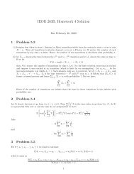
<strong>IEOR</strong><strong>269</strong> notes, Prof. Hochbaum, <strong>2010</strong> 21<br />
(l − 1) + (k − 1) − ∑ e∈P<br />
X e ≤ k + l − (p + 1) − 1<br />
p ≤ ∑ e∈P<br />
X e<br />
⇒ X e = 1 ∀e ∈ P<br />
Done!<br />
Step 2:<br />
There is no fractional tight cycles.<br />
Proof of Step 2: Suppose there were fractional tight cycles in (V, E ∗ ). Consider the one containing<br />
the least number of fractional edges. Each such cycle contains at least two fractional edges e 1 &e 2<br />
(else, the corresponding constraint is not tight).<br />
Let c e1 ≤ c e2 <strong>and</strong> θ = min {1 − X e1 , X e2 }.<br />
The solution {X ′ e} with:<br />
(X ′ e 1<br />
= X e1 + θ), (X ′ e 2<br />
= X e2 − θ) <strong>and</strong> (X ′ e = X e , ∀e ≠ e 1 , e 2 )<br />
is feasible <strong>and</strong> at least as good as the optimal solution {X e }. The feasibility comes from the Lemma<br />
12.3. We are sure that we do not violate any other nontight fractional cycles which share the edge<br />
e 1 . Otherwise, we should have selected θ as the minimum slack on that nontight fractional cycle<br />
<strong>and</strong> update X e accordingly. But, this would incur a solution where two fractional tight cycle share<br />
the fractional edge e ′ 1 which cannot be the case due to Lemma 12.3.<br />
If there were nontight fractional cycles, then we could repeat the same modification for the fractional<br />
edges without violating feasibility. Therefore, there are no fractional cycles in (V, E ∗ ).<br />
The last step to prove that (LP) is the correct form will be to show that the resulting graph is<br />
connected. (Assignment 2)<br />
Lec4<br />
13 Branch-<strong>and</strong>-Bound<br />
13.1 The Branch-<strong>and</strong>-Bound technique<br />
The Branch-<strong>and</strong>-Bound Technique is a method of implicitly (rather than explicitly) enumerating<br />
all possible feasible solutions to a problem.<br />
Summary of LP-based Branch-<strong>and</strong>-Bound Technique (for maximization of pure integer linear programs)<br />
Step 1 Initialization: Begin with the entire set of solutions under consideration as the only remaining<br />
set. Set Z L = −∞. Throughout the algorithm, the best know feasible solution is referred<br />
to as the incumbent solution, <strong>and</strong> its objective value Z L is a lower bound on the maximal