IEOR 263B, Homework 4 Solution
IEOR 263B, Homework 4 Solution
IEOR 263B, Homework 4 Solution

You also want an ePaper? Increase the reach of your titles
YUMPU automatically turns print PDFs into web optimized ePapers that Google loves.
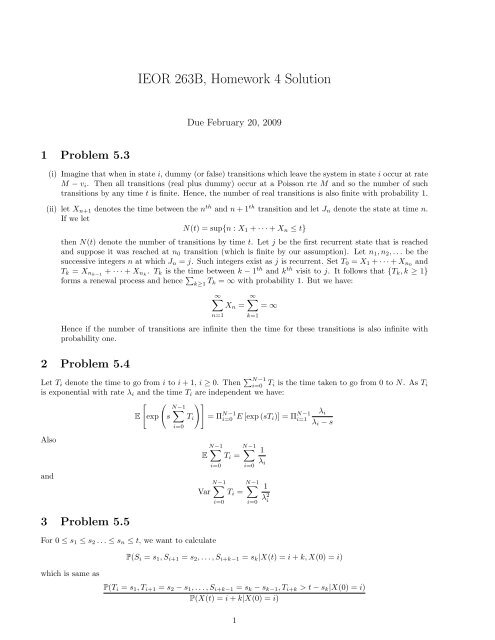
<strong>IEOR</strong> <strong>263B</strong>, <strong>Homework</strong> 4 <strong>Solution</strong><br />
Due February 20, 2009<br />
1 Problem 5.3<br />
(i) Imagine that when in state i, dummy (or false) transitions which leave the system in state i occur at rate<br />
M − v i . Then all transitions (real plus dummy) occur at a Poisson rte M and so the number of such<br />
transitions by any time t is finite. Hence, the number of real transitions is also finite with probability 1.<br />
(ii) let X n+1 denotes the time between the n th and n + 1 th transition and let J n denote the state at time n.<br />
If we let<br />
N(t) = sup{n : X 1 + · · · + X n ≤ t}<br />
then N(t) denote the number of transitions by time t. Let j be the first recurrent state that is reached<br />
and suppose it was reached at n 0 transition (which is finite by our assumption). Let n 1 , n 2 , . . . be the<br />
successive integers n at which J n = j. Such integers exist as j is recurrent. Set T 0 = X 1 + · · · + X n0 and<br />
T k = X nk−1 + · · · + X nk . T k is the time between k − 1 th and k th visit to j. It follows that {T k , k ≥ 1}<br />
forms a renewal process and hence ∑ k≥1 T k = ∞ with probability 1. But we have:<br />
∞∑ ∞∑<br />
X n = = ∞<br />
n=1<br />
Hence if the number of transitions are infinite then the time for these transitions is also infinite with<br />
probability one.<br />
2 Problem 5.4<br />
Let T i denote the time to go from i to i + 1, i ≥ 0. Then ∑ N−1<br />
i=0 T i is the time taken to go from 0 to N. As T i<br />
is exponential with rate λ i and the time T i are independent we have:<br />
Also<br />
and<br />
3 Problem 5.5<br />
E<br />
[<br />
exp<br />
(<br />
s<br />
N−1<br />
∑<br />
i=0<br />
T i<br />
)]<br />
k=1<br />
λ i<br />
= Π N−1<br />
i=0 E [exp (sT i)] = Π N−1<br />
i=1<br />
λ i − s<br />
∑<br />
T i =<br />
N−1<br />
E<br />
i=0<br />
N−1<br />
Var<br />
For 0 ≤ s 1 ≤ s 2 . . . ≤ s n ≤ t, we want to calculate<br />
∑<br />
T i =<br />
i=0<br />
N−1<br />
∑<br />
i=0<br />
N−1<br />
∑<br />
P(S i = s 1 , S i+1 = s 2 , . . . , S i+k−1 = s k |X(t) = i + k, X(0) = i)<br />
i=0<br />
1<br />
λ i<br />
1<br />
λ 2 i<br />
which is same as<br />
P(T i = s 1 , T i+1 = s 2 − s 1 , . . . , S i+k−1 = s k − s k−1 , T i+k > t − s k |X(0) = i)<br />
P(X(t) = i + k|X(0) = i)<br />
1
Using the independence of T m ’s and substituting their densities we get:<br />
iλe −iλs1 (i + 1)λe −(i+1)λ(s2−s1) . . . (i + k − 1)λe −(i+k−1)λ(s i+k−s i+k−1 ) e −(i+k)λ(t−s i+k−1)<br />
( )<br />
i + k − 1<br />
e<br />
i − 1<br />
−λti (1 − e −λt ) k<br />
Simplifying we get:<br />
k!Π k λe −λ(t−sn)<br />
m=1<br />
1 − e −λt<br />
4 Problem 5.12<br />
(i) Since P 0 =<br />
state 0),<br />
1/λ<br />
1/λ + 1/mu = µ , it follows from renewal theory (renewal every time we come back to<br />
λ + µ<br />
N(t)<br />
lim = α 0µ<br />
t→∞ t λ + µ + α 1λ<br />
λ + µ<br />
(ii) The expected total time spent in state 0 by time t is<br />
From this:<br />
E[T 0 (t)] =<br />
∫ t<br />
0<br />
P 00 (s)ds = µ<br />
λ + µ t + λ<br />
(<br />
(λ + µ) 2 1 − e (λ+µ)t)<br />
E[N(t)] = α 0 E[T 0 (t)] + α 1 (t − E[T 0 (t)]).<br />
2