Hedging Quantity Risks with Standard Power Options - UC Berkeley ...
Hedging Quantity Risks with Standard Power Options - UC Berkeley ...
Hedging Quantity Risks with Standard Power Options - UC Berkeley ...
You also want an ePaper? Increase the reach of your titles
YUMPU automatically turns print PDFs into web optimized ePapers that Google loves.
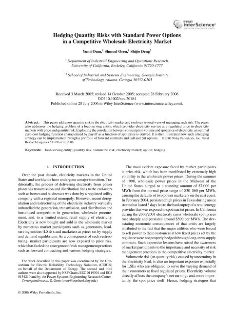
<strong>Hedging</strong> <strong>Quantity</strong> <strong>Risks</strong> <strong>with</strong> <strong>Standard</strong> <strong>Power</strong> <strong>Options</strong><br />
in a Competitive Wholesale Electricity Market<br />
Yumi Oum, 1 Shmuel Oren, 1 Shijie Deng 2<br />
1 Department of Industrial Engineering and Operations Research,<br />
University of California, <strong>Berkeley</strong>, California 94720-1777<br />
2 School of Industrial and Systems Engineering, Georgia Institute<br />
of Technology, Atlanta, Georgia 30332-0205<br />
Received 3 March 2005; revised 14 October 2005; accepted 28 February 2006<br />
DOI 10.1002/nav.20184<br />
Published online 28 July 2006 in Wiley InterScience (www.interscience.wiley.com).<br />
Abstract: This paper addresses quantity risk in the electricity market and explores several ways of managing such risk. The paper<br />
also addresses the hedging problem of a load-serving entity, which provides electricity service at a regulated price in electricity<br />
markets <strong>with</strong> price and quantity risk. Exploiting the correlation between consumption volume and spot price of electricity, an optimal<br />
zero-cost hedging function characterized by payoff as a function of spot price is derived. It is then illustrated how such a hedging<br />
strategy can be implemented through a portfolio of forward contracts and call and put options. © 2006 Wiley Periodicals, Inc. Naval<br />
Research Logistics 53: 697–712, 2006<br />
Keywords:<br />
load-serving entity; quantity risk; volumetric risk; electricity market; option; hedging<br />
1. INTROD<strong>UC</strong>TION<br />
Over the past decade, electricity markets in the United<br />
States and worldwide have undergone a major transition. Traditionally,<br />
the process of delivering electricity from power<br />
plants via transmission and distribution lines to the end-users<br />
such as homes and businesses was done by a regulated utility<br />
company <strong>with</strong> a regional monopoly. However, recent deregulation<br />
and restructuring of the electricity industry vertically<br />
unbundled the generation, transmission, and distribution and<br />
introduced competition in generation, wholesale procurement,<br />
and, to a limited extent, retail supply of electricity.<br />
Electricity is now bought and sold in the wholesale market<br />
by numerous market participants such as generators, loadserving<br />
entities (LSEs), and marketers at prices set by supply<br />
and demand equilibrium. As a consequence of such restructuring,<br />
market participants are now exposed to price risk,<br />
which has fueled the emergence of risk management practices<br />
such as forward contracting and various hedging strategies.<br />
The work described in this paper was coordinated by the Consortium<br />
for Electric Reliability Technology Solutions (CERTS)<br />
on behalf of the Department of Energy. The second and third<br />
authors were also supported by NSF Grants EEC 0119301 and ECS<br />
0134210 and by the <strong>Power</strong> Systems Engineering Research Center.<br />
Correspondence to: S. Oren (oren@ieor.berkeley.edu)<br />
The most evident exposure faced by market participants<br />
is price risk, which has been manifested by extremely high<br />
volatility in the wholesale power prices. During the summer<br />
of 1998, wholesale power prices in the Midwest of the<br />
United States surged to a stunning amount of $7,000 per<br />
MWh from the normal price range of $30–$60 per MWh,<br />
causing the defaults of two power marketers on the east coast.<br />
In February 2004, persistent high prices in Texas during an ice<br />
storm that lasted 3 days led to the bankruptcy of a retail energy<br />
provider that was exposed to spot market prices. In California<br />
during the 2000/2001 electricity crisis wholesale spot prices<br />
rose sharply and persisted around $500 per MWh. The devastating<br />
economic consequences of that crisis are largely<br />
attributed to the fact that the major utilities who were forced<br />
to sell power to their customers at low fixed prices set by the<br />
regulator were not properly hedged through long-term supply<br />
contracts. Such expensive lessons have raised the awareness<br />
of market participants to the importance and necessity of risk<br />
management practices in the competitive electricity market.<br />
Volumetric risk (or quantity risk), caused by uncertainty in<br />
the electricity load, is also an important exposure especially<br />
for LSEs who are obligated to serve the varying demand of<br />
their customers at fixed regulated prices. Electricity volume<br />
directly affects the company’s net earnings and, more importantly,<br />
the spot price itself. Hence, hedging strategies that<br />
© 2006 Wiley Periodicals, Inc.
698 Naval Research Logistics, Vol. 53 (2006)<br />
only concern price risks for a fixed amount of volume cannot<br />
fully hedge market risks faced by LSEs. Unfortunately,<br />
while it is relatively simple to hedge price risks for a specific<br />
quantity (e.g., through forward contracts), such hedging<br />
becomes difficult when the demand quantity is uncertain,<br />
i.e., volumetric risk is involved. When volumetric risks are<br />
involved a company should hedge against fluctuations in<br />
total cost, i.e., quantity times price, but unfortunately, there<br />
are no simple market instruments that would enable such<br />
hedging. Furthermore, a common approach of dealing <strong>with</strong><br />
demand fluctuations for commodities by means of inventories<br />
is not possible in electricity markets where the underlying<br />
commodity is not storable.<br />
The non-storability of electricity combined <strong>with</strong> the<br />
steeply rising supply function and long lead time for capacity<br />
expansion results in strong positive correlation between<br />
demand and price. When demand is high, for instance due to a<br />
heat wave, the spot prices will be high as well and vice versa.<br />
For example, the correlation coefficient between hourly price<br />
and load for 2 years from April 1998 in California 1 was 0.539.<br />
Li and Flynn [20] also calculated the correlation coefficients<br />
between normalized average weekday price and load for 13<br />
markets: for example, 0.70 for Spain, 0.58 for Britain, and<br />
0.53 for Scandinavia. There are some markets where this<br />
price and load relationship is weak but in most markets load<br />
is the most important factor affecting the price of electricity.<br />
The correlation between load and price amplifies the exposure<br />
of an LSE having to serve the varying demand at fixed<br />
regulated prices and accentuates the need for volumetric risk<br />
hedging. An LSE purchasing a forward contract for a fixed<br />
quantity at a fixed price based on the forecasted demand quantity<br />
will find that when demand exceeds its forecast and it is<br />
underhedged, the spot price will be high and most likely will<br />
exceed its regulated sale price, resulting in losses. Likewise,<br />
when demand is low below its forecast, the spot price at which<br />
the LSE will have to settle its surplus will be low and most<br />
likely below its purchase price, again resulting in losses.<br />
Because of the strong causal relationship between electricity<br />
consumption and temperature, weather derivatives have<br />
been considered an effective means of hedging volumetric<br />
risks in the electricity market. The advantage of such<br />
practices stems from the liquidity of weather derivatives<br />
due to their multiple applications. However, the speculative<br />
image of such instruments makes them undesirable<br />
for a regulated utility having to justify its risk management<br />
practices and the cost associated <strong>with</strong> such practices<br />
(which are passed on to customers) to a regulator. In some<br />
1 During this period, all the regulated utilities in the California market<br />
procured electricity from the spot market at the <strong>Power</strong> Exchange<br />
(PX). They were deterred from entering into long-term contracts<br />
through direct limitations on contract prices and disincentives due<br />
to ex post prudence requirements.<br />
jurisdictions, the regulators (e.g., the California Public Utility<br />
Commission (CP<strong>UC</strong>)), who are motivated by concerns<br />
for generation adequacy, require that LSEs hedge their load<br />
serving obligations and appropriate reserves <strong>with</strong> physically<br />
covered forward contracts and options for power. That<br />
is, the hedges cannot just be settled financially or subject<br />
to liquidation damages but must be covered by specific<br />
installed or planned generation capacity capable of physical<br />
delivery. In California, the CP<strong>UC</strong> has explicitly ordered<br />
phasing out of financial contracts <strong>with</strong> liquidation damages<br />
as means of meeting generation adequacy requirements by<br />
2008 [7, 8].<br />
In this paper we propose an alternative to weather derivatives<br />
that involves the use of standard forward electricity contracts<br />
and price-based power derivatives. This new approach<br />
to volumetric hedging exploits the aforementioned correlation<br />
between load and price. Specifically, we address the<br />
problem of developing an optimal hedging portfolio consisting<br />
of forward and options contracts for a risk-averse LSE<br />
when price and volumetric risks are present and correlated.<br />
We derive the optimal payoff function that maximizes the<br />
expected utility of the LSE’s profits and determine the mix<br />
of forwards and options that replicate the optimal payoff of a<br />
hedging portfolio in a single-period setting. While at present<br />
the liquidity of power derivatives is limited, we expect that<br />
better understanding of how such instruments can be used<br />
(which is the goal of this paper) will increase their utilization<br />
and liquidity.<br />
Electricity markets are generally incomplete markets in the<br />
sense that not every risk factor can be perfectly hedged by<br />
market traded instruments. In particular, the volumetric risks<br />
are not traded in electricity markets. Thus, we cannot naively<br />
adopt the classical no-arbitrage approach of constructing a<br />
replicating portfolio for hedging volumetric risks, and the<br />
volumetric risk cannot be eliminated. Since there are a lot of<br />
portfolios of existing derivative contracts that can partially<br />
hedge a given exposure to volumetric risks, the problem is to<br />
select the best one according to some criterion. Our proposed<br />
methodology is based on an alternative approach offered by<br />
the economic literature for dealing <strong>with</strong> risks that are not<br />
priced in the market, by maximizing the expected utility of<br />
economic agents bearing such risks [10, 16, 17].<br />
Our mathematical derivation is based on the utility function<br />
representation of the risk preference of an LSE. We derive an<br />
optimal payoff function that represents payoff as function of<br />
price and <strong>with</strong> zero expected value. We then show how the<br />
optimal payoff function can be synthesized from a portfolio<br />
of forward contracts, European call and put options. We<br />
then provide an example for an LSE considering two alternative<br />
forms of its utility function: (1) constant absolute risk<br />
aversion (CARA) and (2) mean-variance utility risk preference,<br />
under bivariate normal assumptions on the distribution<br />
of quantity and logarithm of price.<br />
Naval Research Logistics DOI 10.1002/nav
Oum, Oren, and Deng: <strong>Hedging</strong> <strong>Quantity</strong> <strong>Risks</strong> 699<br />
<strong>Hedging</strong> problems dealing <strong>with</strong> non-traded quantity risk<br />
have been analyzed in the agricultural literature; farmers also<br />
face correlated price and quantity uncertainty. But the analogy<br />
is imperfect since LSEs have different profit structure,<br />
higher price volatility due to non-storability, and positive<br />
correlation between price and quantity. 2 Furthermore, storage<br />
provides an alternative means for handling quantity risk.<br />
Nevertheless, the farmer’s problem provides some useful references<br />
that are relevant to the LSE’s hedging problem. In a<br />
pioneering article, McKinnon [21] shows that the correlation<br />
between price and quantity is a fundamental feature of<br />
this problem and calculated the variance-optimizing hedge<br />
ratio of futures contracts. He shows that the optimal forward<br />
sale cannot completely eliminate a great deal of uncertainty<br />
that was introduced to the farmer’s income from output<br />
uncertainty. The individual farmer can deal <strong>with</strong> such output<br />
variability by investing in buffer stocks, and McKinnon shows<br />
that buffer stocks can reduce part of quantity uncertainty.<br />
Such storing is not an economical option to consider for the<br />
participants in the electricity market, so LSEs will have to rely<br />
more on financial derivatives. Some articles consider farmers<br />
who find it infeasible to carry buffer stocks from one period<br />
to another [22, 24]. For example, Moschini and Lapan [22]<br />
shows that quantity uncertainty provides a rationale for the<br />
use of options. They derived exact solutions for hedging decisions<br />
on futures and options for a farmer <strong>with</strong> a CARA utility<br />
under multivariate normally distributed price and quantity,<br />
assuming that only one option strike price is available.<br />
With CARA utility function and bivariate normal distribution<br />
for price and quantity, Brown and Toft [3] derives<br />
the optimal payoff that should be acquired by a valuemaximizing<br />
non-financial production firm facing multiplicative<br />
risk of price and quantity. Instead of assuming the<br />
existence of certain instruments, they derive the payoff function<br />
that the optimal portfolio will have. We use their idea<br />
of obtaining the optimal payoff function and solve an LSE’s<br />
problem under different profit, utility, and probability distributions.<br />
Moreover, we extend this approach by replicating<br />
the optimal payoff function using available financial contracts.<br />
Determining the optimal number of contracts from<br />
a set of available options requires solving a difficult optimization<br />
problem, even in a single-period setting, due to<br />
nonlinearity of the option payoff. In this paper we tackle the<br />
problem by first determining a continuous optimal hedging<br />
function and then developing a replicating strategy based on<br />
a portfolio of standard instruments.<br />
Our result shows that we can construct an optimal hedging<br />
portfolio for the LSE that includes forwards and options <strong>with</strong><br />
2 Brown and Toft [3] show that firms <strong>with</strong> the positive price-quantity<br />
correlation should hedge more in most price states to compensate<br />
for the increased exposure associated <strong>with</strong> the positive correlation<br />
than firms <strong>with</strong> the negative price–quantity correlation.<br />
various strike prices. The idea of volumetric hedging using a<br />
spectrum of options was also proposed by Chao and Wilson<br />
[6] from the perspective of a regulator who could impose<br />
such hedging on the LSE as a means of ensuring resource<br />
adequacy and market power mitigation.<br />
The remainder of the paper is organized as follows. In<br />
Section 2, we provide some background about the electricity<br />
market that is relevant to the understanding of volumetric<br />
risks and contracts that can be used to manage volumetric risk.<br />
We also discuss alternative approaches to volumetric risk<br />
management. In Section 3, we explore a way of optimally<br />
utilizing European call and put options in mitigating price<br />
and volumetric risks together. Section 4 concludes the paper.<br />
2. VOLUMETRIC RISKS IN THE<br />
ELECTRICITY MARKET<br />
In electricity markets, an LSE is uncertain about how much<br />
electricity a customer will use at a certain hour until the<br />
customer actually turns a switch on and draws electricity.<br />
Furthermore, the LSE is obligated to provide the customer<br />
<strong>with</strong> electricity whenever it turns the switch on. In other<br />
words, unlike telephone service, there is no busy signal in<br />
electricity supply. Consequently, the electricity demand is<br />
uncertain and thus results in volumetric risks.<br />
Uncertainty or unpredictability of a demand quantity is a<br />
traditional concern for any commodity, but holding inventory<br />
is a good solution to deal <strong>with</strong> quantity risk for those commodities<br />
that can be economically stored. However, electricity<br />
is non-storable, 3 which is the most important characteristic<br />
that differentiates the electricity market from the money market<br />
or other commodities markets. Since electricity needs to<br />
be purchased at the same time it is consumed, the traditional<br />
method of purchasing an excess quantity of a product when<br />
prices are low and holding inventories cannot be used by<br />
the firms retailing electricity. Moreover, unlike other commodities,<br />
LSEs, which are typically regulated, operate under<br />
an obligation to serve and cannot curtail service to their<br />
customers (except under special service agreement) or pass<br />
through high wholesale prices even when they cannot procure<br />
electricity at favorable prices. 4 Consequently, volumetric<br />
risks in the electricity market require special handling.<br />
In the next subsection, we discuss why volumetric risks are<br />
significant in the electricity market. The following subsection<br />
explains financial contracts that can be used to mitigate such<br />
risk.<br />
3 The most efficient way of storing electricity produced is to use<br />
the limited pump capacity installed in some hydro storage plants.<br />
The efficiency of this method is only around 70% [27]. Therefore,<br />
it is generally assumed that electricity is non-storable (at least<br />
economically).<br />
4 In fact, most US states that opened their retail markets to<br />
competition have frozen their retail electricity prices.<br />
Naval Research Logistics DOI 10.1002/nav
700 Naval Research Logistics, Vol. 53 (2006)<br />
2.1. Why Volumetric <strong>Risks</strong> Are Significant to LSEs<br />
Electricity demand is highly affected by local weather condition;<br />
for example, increased need of air conditioners (or<br />
heaters) due to hot (or cold) weather increases electricity<br />
demand. As a result, the load process is volatile, having occasional<br />
spikes caused by extreme weather condition or special<br />
events.<br />
On the other hand, electricity demand is inelastic to price<br />
levels. Currently, most electricity users don’t have incentives<br />
to reduce electricity consumption when spot prices are high<br />
because they face guaranteed fixed prices and LSEs have<br />
an obligation to meet the demand. This price inelasticity<br />
of electricity demand combined <strong>with</strong> the non-storability of<br />
electricity makes sudden spot-price changes more likely than<br />
in any other commodity markets. 5 Consequently, electricity<br />
spot prices exhibit extraordinarily high volatility compared<br />
to financial and commodity markets. For example, the typical<br />
volatility of dollar/yen exchange rates is (10–20%),<br />
LIBOR rates (10–20%), S&P 500 index (20–30%), NASDAQ<br />
(30–50%), natural gas prices (50–100%), while the volatility<br />
of electricity is (100–500% and higher) [12].<br />
Because profits are a function of quantity multiplied by the<br />
price that is extraordinarily volatile and spiky, small uncertainty<br />
in demand volume may become very high uncertainty<br />
in LSEs’ profits. Furthermore, volumetric risks in the electricity<br />
market become severe due to adverse movements of<br />
price and volume: the sales volume is small when the profit<br />
margin is high, while it is large when the margin is low or<br />
even negative. This is due to the price inelasticity of demand<br />
and the resulting strong positive correlation between price<br />
and demand.<br />
2.2. Contracts for Volumetric Risk Management<br />
Due to the non-storability, electricity must be produced<br />
exactly at the same time it is consumed, and electricity supply<br />
and demand must be balanced on a real-time basis; however,<br />
market transactions should occur before the demand and system<br />
constraints are fully known. For this reason, electricity<br />
spot markets have several settlement processes for physical<br />
delivery.<br />
Initial settlement is done in the day-ahead market. The<br />
prices and quantities in the day-ahead market are determined<br />
by matching offers from generators to bids from LSEs by<br />
supply and demand equilibrium, usually for each hour of the<br />
next day. As time approaches to the delivery hour and more<br />
information is revealed on supply and demand conditions,<br />
5 Boisvert et al. [2] and Caves et al. [5] support this argument and<br />
state that price spikes can be mitigated by introducing voluntary<br />
market-based pricing in retail markets. However, regulators have<br />
not been persuaded to adopt market-based real time pricing at the<br />
retail level [15].<br />
additional settlement processes occur in the day-of, hourahead,<br />
and ex post markets, at different prices. 6 However, the<br />
underlying spot price of electricity derivatives is usually the<br />
day-ahead price, because the other markets transacted closer<br />
to delivery than the day-ahead market are designed primarily<br />
for balancing of real-time supply and demand fluctuations.<br />
To manage risks against volatile spot prices for volatile<br />
loads, electricity markets have developed various financial<br />
instruments that can be settled in advance before the spot<br />
market. In this section, we describe various instruments<br />
that can be traded to mitigate volumetric risks: fixed-price<br />
fixed-volume contracts, vanilla options, swing options, interruptible<br />
service contracts, and weather derivatives.<br />
2.2.1. Forward and Futures Contracts<br />
(Fixed-Price Fixed-Volume Contracts)<br />
A simple solution to volumetric risks would be to just settle<br />
a fixed price agreement in advance for a significant amount of<br />
volume. Then, only the remaining amount of demand would<br />
be exposed to the volatile spot prices, resulting in reduced<br />
volumetric risks. This is what forward contracts do.<br />
A forward contract in the electricity market is an agreement<br />
to buy or sell electricity for delivery during a specified period<br />
in the future at a price determined in advance when the contract<br />
is made. In the electricity forward markets, the products<br />
are sold as blocks such as on-peak, off-peak, or super-peak. 7<br />
Forward contracts are over-the-counter (OTC) products.<br />
They need not be standardized; instead, they can be structured<br />
in the most convenient way to the counterparties: they<br />
could be for the delivery to any location during a certain hour,<br />
on-peak or off-peak of a day, week, month, season, or year.<br />
Because of their flexibility, forward contracts are more popular<br />
than futures and are the most liquid and widely used risk<br />
management tool in the electricity market.<br />
Futures contracts are of the same type as forwards, but<br />
they are standardized. In 1996, the New York Mercantile<br />
Exchange (NYMEX) started to trade electricity futures for<br />
6 A day-of market is for the delivery of electricity for the rest of the<br />
day, and an hour-ahead market is for the next couple of hours. Ex<br />
post (or real-time) markets transact for reconciling deviations from<br />
the predicted schedules.<br />
7 On-peak power is the power for peak-load period. In the western<br />
regions of the United States, standard on-peak power in the forward<br />
market is 6 by 16, which means electricity for the delivery from<br />
6:00 to 22:00, Monday through Saturday, excluding North American<br />
Electric Reliability Council (NERC) holidays. On the other hand, in<br />
the eastern and central regions, on-peak power is defined as 5 by 16,<br />
which means electricity for the 16-hour block 6:00 to 22:00, Monday<br />
through Friday, excluding NERC holidays. Super-peak power is the<br />
power for the super-peak period. In the western region, the superpeak<br />
power is 5 by 8, which is for delivery from 12:00 to 20:00,<br />
Monday through Friday. Off-peak power is the power during lowdemand<br />
period, which is the complement to on-peak.<br />
Naval Research Logistics DOI 10.1002/nav
Oum, Oren, and Deng: <strong>Hedging</strong> <strong>Quantity</strong> <strong>Risks</strong> 701<br />
several regions of North America, followed by other exchanges<br />
such as Chicago Board of Trade (CBOT) and the<br />
Minnesota Grain Exchange (MGE) in the United States and<br />
International Petroleum Exchange (IPE) in London. Unfortunately,<br />
for a variety of reasons, after the initial burst of<br />
trading activities, markets in the United States lost their interest<br />
in electricity futures and turned to forward contracts in<br />
OTC markets. As a result, NYMEX, CBOT, and IPE have<br />
stopped their trading of electricity futures. Although MGE is<br />
still trading them, the trading volume is small.<br />
2.2.2. Plain-Vanilla <strong>Options</strong><br />
An option in the electricity markets obligates the issuer<br />
to reimburse the option holder for any positive difference<br />
between the underlying market price and the strike price.<br />
Compared to a contract that specifies a fixed quantity, an<br />
option has the advantage of reducing quantity risks by<br />
enabling an LSE to purchase electricity at the strike price<br />
only when it is needed and the spot price exceeds the strike<br />
price. In particular, a portfolio of call options <strong>with</strong> many different<br />
strike prices would allow the holder to exercise more<br />
options the higher is the spot price, thus obtaining more electricity<br />
when the spot price is higher, which usually occurs<br />
precisely when its load is greater [6].<br />
The electricity options are diverse in contract terms like<br />
products, delivery period, and location. Products could be<br />
on-peak, off-peak, or round-the-clock. The delivery period<br />
could be a month, a quarter, or a year.<br />
The first category of options consists of calendar year and<br />
monthly physical options, which are forward options. The<br />
exercise of the December 2004 call option at the end of<br />
November allows the holder to receive the specified quantity<br />
of electricity (in MWh) during the specified hours (such as<br />
on-peak, off-peak, or round-the-clock hours) of December at<br />
the strike price. In electricity markets, forward options are not<br />
widely traded [11]. The second category of options used in<br />
the electricity market is a strip of daily options. These options<br />
are specified for a given contract period (year, quarter, month,<br />
etc.) and can be exercised daily. For example, the holder of a<br />
December 2004 daily call option can issue an advance notice<br />
on December 15 to receive a specified volume of electricity<br />
on December 16 during the on-peak hours, paying the fixed<br />
price per MWh. Last, there are hourly options for financial<br />
settlements against hourly spot prices during specified blocks<br />
of hours like 1, 4, and 8 hours [14].<br />
2.2.3. Swing <strong>Options</strong><br />
For swing options, the option holder nominates a total<br />
fixed amount to be delivered over the contract period and<br />
is also given the right to swing the volume received <strong>with</strong>in a<br />
certain range, <strong>with</strong> limits on the number of swing right over<br />
the contract period. While a vanilla option protects against<br />
prices for a fixed volume on each day during the delivery<br />
period, a swing option allows the holder to respond to<br />
volumetric risks by adjusting the volume exercised. Accordingly,<br />
the holder can protect more volume when spot prices<br />
are spiky than when spot prices are at a normal level.<br />
Swing options are well studied in the literature, for example:<br />
[9, 15, 18, 26].<br />
2.2.4. Interruptible Service Contracts<br />
Interruptible contracts are made <strong>with</strong> customers who are<br />
willing to have their electricity service interrupted by the LSE<br />
under specified conditions. In exchange for the interruption<br />
option, the LSE typically offers a lower electricity rate to the<br />
customer. In the situations where supply or demand shocks<br />
occur, the interruptible contracts allow LSEs to interrupt the<br />
counterparty’s service at a lower cost than serving them by<br />
purchasing power at the high spot price. For literature on such<br />
contracts, see [12, 25].<br />
2.2.5. Weather Derivatives<br />
Weather derivatives give payouts depending on the realized<br />
weather variables; thus, they can be used to hedge volumetric<br />
risks for various industries whose supply and demand<br />
volume is affected by weather conditions. Since the first<br />
transaction by energy companies took place in 1997, the<br />
transaction volume in weather derivatives has been expanding<br />
rapidly among diverse industries such as agriculture,<br />
tourism, beverage, ice cream, and entertainment. In addition,<br />
weather derivatives are used by investment firms as independent<br />
means of diversifying their risks from the existing<br />
financial markets because it is widely perceived that the correlations<br />
between weather indices and most financial indices<br />
are negligible.<br />
Traditionally, hedging against abnormal weather conditions<br />
has been done through insurance contracts. These<br />
insurance contracts are typically settled to cover against catastrophic<br />
weather conditions such as drought and floods.<br />
However, these contracts cannot protect against abnormal but<br />
less extreme weather conditions, which could also affect profits.<br />
The need for an instrument that can be used to hedge such<br />
non-catastrophic weather conditions brought the weather<br />
derivatives into the market. Moreover, for weather derivatives,<br />
there is no need to provide proofs of financial loss to<br />
receive payout unlike insurance contracts; payoffs of weather<br />
derivatives are decided by the actual weather readings at a<br />
weather station specified in the contract.<br />
Among the various weather derivatives in use based on<br />
indices such as precipitation, temperature, and wind speed,<br />
Naval Research Logistics DOI 10.1002/nav
702 Naval Research Logistics, Vol. 53 (2006)<br />
the most commonly traded weather derivatives are Heating<br />
Degree Days (HDD) and Cooling Degree Days (CDD)<br />
derivatives. The HDD (CDD) index is the sum of positive<br />
values of average temperature 8 minus 65 ◦ during the contract<br />
period, mostly a month or a season. The reason for the<br />
popularity of degree-days derivatives is not only the transparency<br />
of the data and value, but also the high correlation<br />
between electricity demand and degree-days. In response<br />
to the increased demand, Chicago Mercantile Exchange<br />
(CME) started a standard electronic market place for HDD<br />
and CDD futures and options since September 1999 now<br />
reaching a more than 30,000 annual trading volume. 9 They<br />
are also traded in OTC markets such as LIFFE (London<br />
International Financial Futures and <strong>Options</strong> Exchange)<br />
and electronic market places like ICE (intercontinental<br />
Exchange).<br />
Suppose an LSE decides to mitigate its volumetric risk<br />
associated <strong>with</strong> serving the uncertain electricity demand in its<br />
service area during winter. If the upcoming winter is mild, the<br />
electricity demand would be low, leaving the LSE <strong>with</strong> low<br />
revenue. Using the fact that the electricity demand increases<br />
as the HDD value increases in the LSE’s service area, the<br />
LSE could buy an HDD put option <strong>with</strong> strike 2500 and tick<br />
amount 10 $10, for instance. If the upcoming winter were mild<br />
and the HDD were 2000, then the LSE would receive $5000.<br />
However, if the realized HDD were greater than the strike<br />
value, 2500, then no payout is made from the contracts. In<br />
this way, the LSE would offset its low revenues when the<br />
weather is unfavorable.<br />
2.2.6. <strong>Power</strong>-Weather Cross-commodity Derivatives<br />
Since the price risk and volumetric risk are correlated,<br />
weather derivatives that only cover the volumetric risk would<br />
not be effective <strong>with</strong>out additional hedging of price risk. For<br />
example, LSEs definitely don’t like the cases where load<br />
is too high at the same time as the wholesale price spikes.<br />
But if the wholesale price is not very high, then the high<br />
load would be generally favorable to them. Such LSEs can<br />
benefit from the power–weather derivatives that would give<br />
positive payouts when two conditions are both met, for example,<br />
whenever temperature is above 80 ◦ at the same time as<br />
the spot price of electricity is above $100. The merit of this<br />
kind of double-triggered cross-commodity derivatives is that<br />
they are cheaper than the standard weather derivatives. They<br />
are available in OTC markets and provide efficient tools for<br />
volumetric risk management for LSEs.<br />
8 Mean of maximum and minimum temperature of the day.<br />
9 [source: www.cme.com].<br />
10 The tick amount is the money that the put option would payout<br />
for one unit of HDD deviation under the strike price.<br />
3. OPTIMALLY HEDGING VOLUMETRIC<br />
RISKS USING STANDARD CONTRACTS<br />
While weather derivatives can be used to mitigate volumetric<br />
risks because of the high correlation between power<br />
demand and weather variables, appropriate use of power<br />
derivatives would also help in mitigating volumetric risks<br />
due to the correlation between power demand and price.<br />
The use of standard electricity instruments may be advantageous<br />
when an LSE needs to avoid the speculative stigma<br />
of weather derivatives. Regulators may view weather derivative<br />
trading as a speculative activity and be reluctant to allow<br />
the LSE to pass the cost of such risk management tactics to<br />
consumers served at regulated rates. Weather derivatives do<br />
nothing to insure supply adequacy, which is a major concern<br />
in the power industry. As mentioned earlier, concerns<br />
for generation adequacy have motivated regulators to require<br />
that LSEs hedge their load serving obligations and reserves<br />
<strong>with</strong> contracts that are covered by physical generation<br />
capacity.<br />
In this section, we propose a new approach for managing<br />
volumetric risks by constructing a portfolio of standard forward<br />
contracts and power derivatives whose underlying is the<br />
wholesale electricity spot price. If needed, such instruments<br />
can be backed by physical generation capacity or interruptible<br />
supply contracts that will assure deliverability of the hedged<br />
energy.<br />
Consider an LSE who is obligated to serve an uncertain<br />
electricity demand q at the fixed price r. Assume that the<br />
LSE procures electricity that it needs in order to serve its<br />
customers from the wholesale market at spot price p.<br />
To protect against price risk, the LSE can enter into forward<br />
contracts to fix the buying price at the forward price F . First,<br />
the number of forward contracts to be purchased needs to<br />
be determined. Suppose that the LSE decides to purchase<br />
an amount ¯q of forwards; then, the actual demand would be<br />
¯q + q. Then, the profit that is at risk is q · (r − p). The<br />
LSE would want to protect against the situation where either<br />
spot price p is higher than r and q > 0orp is less than r<br />
and q < 0. Now the second question arises: how to manage<br />
this remaining risk?<br />
The LSE’s strategy could be buying call options <strong>with</strong> strike<br />
prices that are higher than r and exercised when q > 0 and<br />
buying put options <strong>with</strong> strike prices less than r and exercised<br />
when q < 0. Of course, prices of the call/put options are<br />
not negligible. Then, the relevant decision problem is to determine<br />
how many put/call options should the LSE purchase and<br />
at what strike prices?<br />
The timing of entering into forward and options contracts<br />
is also an important decision, since the forward and<br />
options prices change as the time approaches the delivery<br />
period, reflecting the changing expectations in the market.<br />
Optimizing such timing decisions requires solving an<br />
Naval Research Logistics DOI 10.1002/nav
Oum, Oren, and Deng: <strong>Hedging</strong> <strong>Quantity</strong> <strong>Risks</strong> 703<br />
integrated problem of selecting the optimal hedging portfolio<br />
and choosing the optimal timing of purchase. However, the<br />
timing problem is out of the scope of this paper. 11 Here we<br />
restrict ourselves to a single period model where a hedging<br />
portfolio is constructed at time 0 in order to reduce risk from<br />
serving retail load at time 1. A single-period model will allow<br />
us to see the implications of the optimal hedging strategy.<br />
To deal <strong>with</strong> this hedging problem, we first derive the overall<br />
payoff that the optimal hedging portfolio should have as a<br />
function of realized spot price p and then determine how to<br />
span this payoff <strong>with</strong> forwards and options.<br />
where E[·] and E Q [·] denote expectations under the probability<br />
measure P and Q, respectively. In (2), we require<br />
the manufacturing cost 12 of the portfolio to be zero under<br />
a constant risk-free rate. This zero-cost constraint implies<br />
that purchasing derivative contracts may be financed from<br />
selling other derivative contracts or from the money market<br />
accounts. In other words, under the assumption that there is no<br />
limits on the possible amount of instruments to be purchased<br />
and money to be borrowed, our model finds a portfolio from<br />
which the LSE obtains the maximum expected utility over<br />
total profit.<br />
3.1. Obtaining the Optimal Payoff Function<br />
3.1.1. Mathematical Formulation<br />
In our single-period setting, hedging instruments are purchased<br />
at time 0 and all payoffs are received at time 1.<br />
<strong>Hedging</strong> portfolio has an overall payoff structure x(p), which<br />
depends on the realization of the spot price p at time 1.<br />
Note that our hedging portfolio may include money market<br />
accounts, letting the LSE borrow money to finance hedging<br />
instruments. Let y(p, q) be the LSE’s profit from serving<br />
the load at the fixed rate r at time 1. Then, the total profit<br />
Y(p, q, x(p)) after receiving payoffs from the contracts in<br />
the hedging portfolio is given by<br />
where<br />
Y(p, q, x(p)) = y(p, q) + x(p), (1)<br />
y(p, q) = (r − p)q.<br />
The LSE’s preference is characterized by a concave utility<br />
function U defined over the total profit Y(·) at time 1. LSE’s<br />
beliefs on the realization of spot price p and load q are characterized<br />
by a joint probability function f(p, q) for positive<br />
p and q, which is defined on the probability measure P .On<br />
the other hand, let Q be a risk-neutral probability measure<br />
by which the hedging instruments are priced and g(p) be the<br />
probability density function of p under Q. Because the electricity<br />
market is incomplete, there may exist infinitely many<br />
risk-neutral probability measures. We assume that a specific<br />
measure Q was picked according to some optimal criteria.<br />
We formulate the LSE’s problem as<br />
max<br />
x(p)<br />
E[U[Y(p, q, x(p))]]<br />
s.t. E Q [x(p)]=0, (2)<br />
3.1.2. Optimality Conditions<br />
The Lagrangian function for the above constrained optimization<br />
problem is given by<br />
L(x(p)) = E[U(Y(p, q, x(p)))]−λE Q [x(p)]<br />
=<br />
∫ ∞<br />
−∞<br />
E[U(Y)|p]f p (p)dp − λ<br />
∫ ∞<br />
−∞<br />
x(p)g(p)dp<br />
<strong>with</strong> a Lagrange multiplier λ and the marginal density function<br />
f p (p) of p under P . Differentiating L(x(p)) <strong>with</strong> respect<br />
to x(·) results in<br />
[ ]<br />
∂L ∂Y<br />
∂x(p) = E ∂x U ′ (Y )<br />
∣ p f p (p) − λg(p) (3)<br />
by the Euler equation. Setting (3) to zero and substituting<br />
∂Y<br />
= 1 from (1) yields the first-order condition for the<br />
∂x<br />
optimal solution x ∗ (p) as follows:<br />
E[U ′ (Y (p, q, x ∗ (p)))|p] =λ ∗ g(p)<br />
f p (p) . (4)<br />
Here, the value of λ ∗ should be the one that satisfies the zerocost<br />
constraint (2). If g(p) = f p (p) for all p, then (4) implies<br />
that the optimal payoff function makes an expected marginal<br />
utility from the variation in q to be the same for any p.<br />
3.1.3. CARA Utility<br />
A CARA utility function has an exponential form: U(Y) =<br />
− 1 a e−aY where a is the coefficient of absolute risk aversion.<br />
With CARA utility, the optimal payoff function x ∗ (p), which<br />
11 Related work on this topic can be found in [23], which considers<br />
the optimal timing of static hedges using only forward contracts.<br />
12 A derivative price is an expected value of the discounted payoff<br />
under the risk-neutral measure Q.<br />
Naval Research Logistics DOI 10.1002/nav
704 Naval Research Logistics, Vol. 53 (2006)<br />
satisfies (4), is obtained as<br />
x ∗ (p) = 1 a<br />
− 1 a<br />
(<br />
ln f p(p)<br />
)<br />
g(p) + ln E[e−ay(p,q) |p]<br />
(E Q [<br />
ln f p(p)<br />
g(p)<br />
]<br />
+ E Q [ln E[e −ay(p,q) |p]]<br />
)<br />
. (5)<br />
PROOF: We see from the special property U ′ (Y ) =<br />
−aU(Y ) of a CARA utility function that the following<br />
condition holds:<br />
E[U(Y ∗ )|p] =− λ∗<br />
a<br />
g(p)<br />
f p (p) ,<br />
which implies that the utility which is expected at any price<br />
level p is proportional to g(p)<br />
f p<br />
. Then the optimal condition<br />
(p)<br />
is reduced to<br />
E[e −a(y(p,q)+x∗ (p)) |p] =λ ∗ g(p)<br />
f p (p)<br />
for an LSE <strong>with</strong> a CARA utility function. Then,<br />
x ∗ (p) = 1 ( )<br />
1<br />
a ln f p (p)<br />
λ ∗ g(p) E[e−ay(p,q) |p]<br />
= 1 (<br />
− ln λ ∗ + ln f )<br />
p(p)<br />
a<br />
g(p) + ln E[e−ay(p,q) |p] . (6)<br />
The Lagrange multiplier λ ∗ in the equation should satisfy the<br />
zero-cost constraint (2), which is ∫ ∞<br />
−∞ x∗ (p)g(p)dp = 0.<br />
That is,<br />
∫ ∞<br />
−∞<br />
(<br />
1<br />
− ln λ ∗ + ln f p(p)<br />
a<br />
g(p)<br />
)<br />
+ ln E[e −ay(p,q) |p] g(p)dp = 0. (7)<br />
Solving (7) for ln λ ∗ gives<br />
ln λ ∗ =<br />
∫ ∞<br />
−∞<br />
(<br />
ln f )<br />
p(p)<br />
g(p) + ln E[e−ay(p,q) |p] g(p)dp.<br />
Substituting this into Eq. (6) gives the optimal solution (5).<br />
□<br />
3.1.4. Mean-Variance Approach<br />
The mean-variance approach is to maximize a meanvariance<br />
objective function, which is linearly increasing<br />
in the mean and decreasing in the variance of the profit:<br />
E[U(Y)]=E[Y ]− 1 aV ar(Y). It follows from Var(Y)=<br />
2<br />
E[Y 2 ]−E[Y ] 2 that<br />
U(Y) ≡ Y − 1 2 a(Y 2 − E[Y ] 2 )<br />
for the mean-variance objective function in an expected utility<br />
form. Then, the optimal solution x ∗ (p) that satisfies (4) is<br />
obtained as<br />
(<br />
x ∗ (p) = 1 g(p) )<br />
f p (p)<br />
1 −<br />
a E Q[ g(p)<br />
] − E[y(p, q)|p]<br />
f p (p)<br />
+ E Q [E[y(p, q)|p]]<br />
g(p)<br />
f p (p)<br />
E Q[ g(p)<br />
f p (p)<br />
]. (8)<br />
PROOF: From U ′ (Y ) = 1 − aY, the optimal condition (4)<br />
is as follows:<br />
Equivalently,<br />
E[1 − aY ∗ |p] =λ ∗ g(p)<br />
f p (p) .<br />
f p (p) − aE[Y ∗ |p]f p (p) = λ ∗ g(p). (9)<br />
Integrating both sides <strong>with</strong> respect to p from −∞ to ∞, we<br />
obtain λ ∗ = 1−aE[Y ∗ ]. Substituting λ ∗ and Y ∗ = y(p, q)+<br />
x ∗ (p) into (9) gives<br />
f p (p) − a(E[y(p, q)|p]+x ∗ (p))f p (p)<br />
= g(p) − a(E[y(p, q)]+E[x ∗ (p)])g(p).<br />
By rearranging, we obtain<br />
x ∗ (p) = 1 a − 1 a<br />
g(p)<br />
f p (p) + (E[y(p, q)]+E[x∗ (p)])<br />
× g(p) − E[y(p, q)|p]. (10)<br />
f p (p)<br />
To cancel out E[x ∗ (p)] in the right-hand side, we take the<br />
expectation under Q to the both sides to obtain<br />
0 = 1 a − 1 [ ] g(p)<br />
a EQ + (E[y(p, q)]+E[x ∗ (p)])<br />
f p (p)<br />
× E Q [ g(p)<br />
f p (p)<br />
]<br />
− E Q [E[y(p, q)|p]], (11)<br />
Naval Research Logistics DOI 10.1002/nav
Oum, Oren, and Deng: <strong>Hedging</strong> <strong>Quantity</strong> <strong>Risks</strong> 705<br />
g(p)/f p(p)<br />
and subtract Eq. (11) ×<br />
E Q [g(p)/f p<br />
from Eq. (10). This<br />
(p)]<br />
gives the final formula for the optimal payoff function under<br />
mean-variance utility as in (8).<br />
□<br />
Note that when we can assume P ≡ Q in the electricity<br />
market, which was empirically justified in [1, 19] for<br />
the Nordic electricity forward market, the optimal payoff<br />
function under the mean-variance utility becomes<br />
x ∗ (p) = E[y(p, q)]−E[y(p, q)|p]. (12)<br />
The first term E[y(p, q)] is a constant, and the second term<br />
E[y(p, q)|p] is the expected profit given the value of the spot<br />
price. This implies that whatever the spot price is realized,<br />
the optimal portfolio is the one that makes the expected total<br />
profit for any given price under quantity uncertainty to be the<br />
same as the expected profit before hedging. This is because<br />
maximizing the mean-variance objective function <strong>with</strong> our<br />
zero-cost constraint and P ≡ Q is the same as just minimizing<br />
a variance of profit after hedging. 13 In fact, given<br />
the value of p, the variance of profit is zero after adding the<br />
optimal payoff in (12). We see that the optimal portfolio can<br />
remove only the uncertainty in revenue that is correlated <strong>with</strong><br />
price.<br />
3.1.5. Bivariate Lognormal-Normal Distribution<br />
for Price and Load<br />
Suppose the marginal distributions of p and q as follows:<br />
Under P : log p ∼ N(m 1 , s 2 ), q ∼ N(m, u 2 ),<br />
Corr(log p, q) = ρ<br />
Under Q : log p ∼ N(m 2 , s 2 ).<br />
Then, we can get the explicit functions for the optimal payoff.<br />
For the CARA utility, the optimal payoff function (5)<br />
reduces to<br />
where<br />
x ∗ (p) = 1 a (A 1(p) + A 2 (p)), (13)<br />
A 1 (p) ≡ ln f [<br />
p(p)<br />
g(p) − EQ ln f ]<br />
p(p)<br />
=− m 2 − m 1<br />
(log p − m<br />
g(p) s 2 2 )<br />
A 2 (p) ≡ ln E[e −ay(p,q) |p]−E Q [ln E[e −ay(p,q) |p]]<br />
=−arρ u (<br />
s (log p − EQ [log p]) + a m − ρ u )<br />
s m 1 (p − E Q [p]) + aρ u s (p log p − EQ [p log p])<br />
+ 1 2 a2 (−2r(p − E Q [p]) + p 2 − E Q [p 2 ])u 2 (1 − ρ 2 )<br />
=−arρ u (<br />
s (log p − m 2) + a m − ρ u ) (p<br />
s m 1 − e<br />
m 2<br />
)<br />
+<br />
u<br />
1<br />
2 s2 + aρ<br />
(p log p − (m 2 + s 2 )e m 2+ 1 s2) 2<br />
s<br />
+ 1 2 a2( −2r(p − e m 2+ 1 2 s2 )<br />
+ p 2 − e 2m 2+2s 2 )<br />
u 2 (1 − ρ 2 )<br />
13 This kind of hedging is also considered in [11]: mean-variance<br />
hedging reduces to variance minimization when the pricing<br />
measure equals to the physical measure because they consider<br />
only forward contracts, which have zero expected value before<br />
delivery.<br />
and for the mean-variance utility, the optimal payoff function<br />
(8) reduces to<br />
x ∗ (p) = 1 a (1 − B 1(p)) − B 2 (p) + B 3 B 1 (p), (14)<br />
Naval Research Logistics DOI 10.1002/nav
706 Naval Research Logistics, Vol. 53 (2006)<br />
where<br />
B 1 (p) ≡<br />
g(p) (<br />
f p (p)<br />
m2 − m 1<br />
E Q[ g(p)<br />
] = exp log p + m2 1 − m2 2<br />
− (m 1 − m 2 ) 2 )<br />
s 2 2s 2 s 2 f p (p)<br />
= e − (m 1 −m 2 )(m 1 −3m 2 )<br />
2s 2 p m 2 −m 1<br />
s 2<br />
B 2 (p) ≡ E[y(p, q)|p] =E[(r − p)q|p] =(r − p)<br />
(<br />
m + ρ u )<br />
s (log p − m 1)<br />
B 3 ≡ E Q [E[y(p, q)|p]]<br />
(<br />
= (r − E Q [p]) m − ρ u )<br />
s m 1 + ρ u s (rEQ [log p]−E Q [p log p])<br />
= ( r − e m ) ( 2+ 1 2 s2 m − ρ u )<br />
s m 1 + ρ u (<br />
rm2 − (m 2 + s 2 )e m )<br />
2+ 1 2 s2 .<br />
s<br />
We have used the following formulas in the calculation.<br />
E Q [log p] =m 2<br />
E Q [p] =e m 2+ 1 2 s2<br />
E Q [p log p] =(m 2 + s 2 )e m 2+ 1 2 s2<br />
E Q [p 2 ]=e 2m 2+2s 2<br />
1<br />
(−<br />
g(p)<br />
f p (p) = ps √ sπ exp 1 2<br />
1<br />
ps √ sπ exp (− 1 2<br />
( ) ) 2 log p−m2<br />
s<br />
(<br />
log p−m1<br />
s<br />
) 2<br />
) = exp<br />
(<br />
m2 − m 1<br />
log p + m2 1 − )<br />
m2 2<br />
s 2 2s 2<br />
[ ] ( g(p)<br />
E Q m2 − m 1<br />
= exp m<br />
f p (p)<br />
s 2 2 + m2 1 − m2 2<br />
+ (m 2 − m 1 ) 2 ) ( (m1 − m 2 ) 2 )<br />
= exp<br />
2s 2 2s 2 s 2<br />
We’ve also used q|p ∼ N ( m + ρ u s (log p − m 1), u 2 (1 − ρ 2 ) )<br />
to obtain<br />
Then, we can get the explicit functions for the optimal payoff<br />
for the mean-variance utility:<br />
ln E[e −ay(p,q) |p] ≡ln E[e −a(r−p)q |p]<br />
(<br />
=−a(r − p) m + ρ u )<br />
s (log p − m 1)<br />
+ 1 2 a2 (r − p) 2 u 2 (1 − ρ 2 ).<br />
3.1.6. Bivariate Lognormal Distribution<br />
for Price and Load<br />
Suppose the marginal distributions of p and q, on the other<br />
hand, follow bivariate lognormal distributions as follows:<br />
Under P : log p ∼ N(m 1 , s 2 ), log q ∼ N ( m q , uq) 2 ,<br />
Corr(log p, log q) = φ<br />
Under Q : log p ∼ N(m 2 , s 2 ).<br />
Naval Research Logistics DOI 10.1002/nav<br />
where<br />
x ∗ (p) = 1 a (1 − B 1(p)) − B ′ 2 (p) + B′ 3 B 1(p), (15)<br />
B 2 ′ (p) ≡ E[y(p, q)|p] =E[(r − p)q|p]<br />
= (r − p)e m q+φ uq s (log p−m 1)+ 1 2 u2 q (1−φ2 )<br />
since log q|p ∼ N(m q + φ u q<br />
s (log p − m 1), u 2 q (1 − φ2 )), and<br />
B ′ 3 ≡ EQ [E[y(p, q)|p]]<br />
= re m q+φ uq s (m 2−m 1 )+ 1 2 u2 q (1−φ2 )+ 1 2 φ2 u2 q<br />
s 2 s2<br />
− e m 2+m q +φ uq s (m 2−m 1 )+ 1 2 u2 q (1−φ2 )+ 1 2 (φ uq s +1)2 s 2 . (16)
Oum, Oren, and Deng: <strong>Hedging</strong> <strong>Quantity</strong> <strong>Risks</strong> 707<br />
3.2. Replicating the Optimal Payoff Function<br />
In the previous section, we’ve obtained the payoff function<br />
x ∗ (p) that the optimal portfolio should have. In this section,<br />
we construct a portfolio that replicates payoff x(p).<br />
In [4], Carr and Madan showed that any twice continuously<br />
differentiable function x(p) can be written in the following<br />
form:<br />
x(p) =[x(s) − x ′ (s)s]+x ′ (s)p +<br />
+<br />
∫ s<br />
0<br />
∫ ∞<br />
s<br />
x ′′ (K)(K − p) + dK<br />
x ′′ (K)(p − K) + dK<br />
for an arbitrary positive s. This formula suggests a way of<br />
replicating payoff x(p). Let F be the forward price for a<br />
delivery at time 1. Evaluating the equation at s = F and<br />
rearranging it gives<br />
∫ F<br />
x(p) = x(F)· 1 + x ′ (F )(p − F)+ x ′′ (K)(K − p) + dK<br />
+<br />
∫ ∞<br />
F<br />
0<br />
x ′′ (K)(p − K) + dK. (17)<br />
Note that 1, (p − F), (K − p) + , and (p − K) + in the above<br />
expression represent payoffs at time 1 of a bond, forward<br />
contract, put option, and call option, respectively.<br />
Therefore,<br />
x(F) units of bonds,<br />
x ′ (F ) units of forward contracts,<br />
x ′′ (K)dK units of put options <strong>with</strong> strike K for every<br />
KF<br />
gives the same payoff as x(p).<br />
The above implies that unless the optimal payoff function<br />
is linear, the optimal strategy involves purchasing (or selling<br />
short) a spectrum of both call and put options <strong>with</strong> continuum<br />
of strike prices. This result proves that LSEs should<br />
purchase a portfolio of options to hedge price and quantity<br />
risk together. Even if prices go up <strong>with</strong> increasing loads, more<br />
call options <strong>with</strong> higher strike prices are exercised, having an<br />
effect of putting price caps on each incremental load.<br />
In practice, electricity derivatives markets, as any derivatives<br />
markets, are incomplete. Consequently, the market does<br />
not offer options for the full continuum of strike prices, but<br />
typically only a small number of strike prices are offered.<br />
Our purpose is to best replicate the optimal payoff function<br />
using existing options only. Therefore, we need to decide<br />
what amount of options to purchase for each available strike<br />
price so that the total payoff from those options is equal or<br />
close to the payoff provided by the optimal payoff function.<br />
Let K 1 , ..., K n be available strike prices for put options and<br />
K<br />
1 ′ , ..., K′ m be available strike prices for call options where<br />
0
708 Naval Research Logistics, Vol. 53 (2006)<br />
3.3. An Example<br />
In this section, we illustrate the method that we derived<br />
in the previous sections. We consider the on-peak hours of<br />
a single summer day as time 1. Parameters were approximately<br />
based on the California <strong>Power</strong> Exchange data of<br />
daily day-ahead average on-peak prices and 1% of the total<br />
daily on-peak loads from July to September 1999. Specific<br />
parameter values are imposed as follows:<br />
• Price is distributed lognormally <strong>with</strong> parameters<br />
m1 = 3.64 and s = 0.35 in both the real-world<br />
and risk-neutral world: log p ∼ N(3.64, 0.35 2 ) in<br />
P and Q. The expected value of the price p under<br />
this distribution is $40.5/MW h.<br />
• The fixed rate r = $100/MW h is charged to the<br />
customers who are served by the LSE.<br />
• For CARA utility, the risk aversion is a = 1.5.<br />
• Load is either normally distributed <strong>with</strong> mean m =<br />
300 and u 2 = 30 2 or lognormally distributed <strong>with</strong><br />
parameter m = 5.77 and u = 0.09.<br />
We would like to point out a significant correlation effect<br />
in the profit distributions. Figure 1 shows that the profit distributions<br />
become quite different as the correlation between<br />
load and logarithm of price changes. Considering that the correlation<br />
coefficient of our data is 0.7, we observe that the correlation<br />
coefficient cannot be ignored in the analysis of profit.<br />
The optimal payoff functions for a CARA utility LSE<br />
are drawn in Figure 2 for various correlation coefficients<br />
between log p and q. Generally, low profit from high loads for<br />
Figure 1. Profit distribution for various correlation coefficients.<br />
Generated 50,000 pairs of (p, q) from a bivariate normal distribution<br />
of (log p, q) <strong>with</strong> a various correlation ρ’s, where log p ∼<br />
N(3.64, 0.35 2 ) and q ∼ N(300, 30 2 ) and plotted estimated probability<br />
density functions of the profit using normal kernel (assuming<br />
r = $100/MW h). [Color figure can be viewed in the online issue,<br />
which is available at www.interscience.wiley.com.]<br />
Figure 2. The optimal payoff function for an LSE <strong>with</strong> CARA<br />
utility when price and load follow bivariate lognormal-normal distribution<br />
log p ∼ N(3.64, 0.35 2 ) and q ∼ N(300, 30 2 ) <strong>with</strong> correlation<br />
coefficient ρ. [Color figure can be viewed in the online issue, which<br />
is available at www.interscience.wiley.com.]<br />
very high spot prices and from low load for very low spot price<br />
is compensated <strong>with</strong> the cases where spot prices and loads are<br />
around the expected value. This can be seen from the graph<br />
where as the spot price goes away from r, positive payoff is<br />
received from the optimal portfolio while the payoff is negative<br />
around r. We also note that larger payoff can be received<br />
when the correlation is smaller. This is because the variance<br />
of profit is bigger when the correlation is smaller, as we can<br />
see from Figure 1. Therefore, even when the correlation is<br />
zero, the optimal payoff function is nonlinear.<br />
Figure 3 illustrates the numbers of contracts to be purchased<br />
in order to obtain the payoff x ∗ (p) for an LSE <strong>with</strong> a<br />
CARA utility function. We see that the numbers of options<br />
contracts are very high relative to the mean volume. This<br />
is because we don’t restrict the model <strong>with</strong> constraints such<br />
as credit limits. The zero-cost constraint (2) that we only<br />
included in our model enables borrowing as much money as<br />
needed to finance any number of derivative contracts.<br />
For an LSE <strong>with</strong> mean-variance utility, the optimal payoff<br />
functions are drawn in Figure 4. They show the tendency of<br />
mean-variance utility to protect against high price and low<br />
quantity. For an illustration of the numbers of contracts to be<br />
purchased in order to obtain payoff x ∗ (p), see Figure 5. Note<br />
that in our examples the number of options contracts to be<br />
purchased in the optimal portfolio is positive for any strike<br />
prices. This implies that we borrow money from the bank and<br />
purchase a portfolio of options contracts.<br />
Figure 6 compares distribution changes between profit<br />
<strong>with</strong>out hedging, profit after price hedge 14 and profit after<br />
14 Price hedge here means that we add the optimal payoff function<br />
obtained under the assumption of no quantity risk. This is in fact<br />
equivalent to buying forwards for the average load quantity.<br />
Naval Research Logistics DOI 10.1002/nav
Oum, Oren, and Deng: <strong>Hedging</strong> <strong>Quantity</strong> <strong>Risks</strong> 709<br />
Figure 3. The graphs show numbers of forward and options contracts to be purchased in order to replicate the optimal payoff x ∗ (p) that<br />
is obtained for the LSE <strong>with</strong> CARA utility. In this example, the forward price is $40.5/MWh, thus, the optimal portfolio includes forward<br />
contracts for x ′ (40.5) MWh, put options on x ′′ (K)dK MWh for K40.5. [Color figure<br />
can be viewed in the online issue, which is available at www.interscience.wiley.com.]<br />
the optimal price and quantity hedge. 15 The graphs shows<br />
significant improvements in reducing risks when we hedge<br />
price and quantity risk together.<br />
In Figure 7 we explore the sensitivity of the optimal<br />
payoff function <strong>with</strong> respect to the divergence between<br />
the risk-neutral distribution and the assumed physical distribution<br />
of prices. Specifically, we assume that the joint<br />
distribution for quantity and price under both measures P<br />
and Q is represented by a bivariate lognormal-normal density<br />
function <strong>with</strong> possible differences in the mean logarithmic<br />
price, which we vary. The results depend on the utility function<br />
used. For CARA utility, the overall payoff is higher than<br />
15 Price and quantity hedge refers to the optimal payoff function that<br />
we obtained in this paper.<br />
the optimal payoff if the expected price is higher than the<br />
market price, but the difference is not that significant <strong>with</strong><br />
respect to the payoff changes for differing p. For the meanvariance<br />
case, however, the difference between payoffs for<br />
varying mean logarithmic price m 2 is more noticeable.<br />
Figure 8 shows how hedging strategies change <strong>with</strong> risk<br />
aversion. Figure 8a displays the optimal payoff functions for<br />
CARA utility <strong>with</strong> different levels of risk aversion. It shows<br />
that the payoff function <strong>with</strong> high risk aversion is more sensitive<br />
to the unit change in spot price, indicating that a more<br />
risk averse LSE will enter into more active hedging. On the<br />
other hand, mean-variance utility shows different aspects.<br />
In Figure 8b, as a gets close to 0.01, the optimal payoff<br />
doesn’t change much; the mean-variance objective function<br />
gives more weight to variance as a gets bigger, so a won’t<br />
Figure 4. Optimal payoff functions for an LSE <strong>with</strong> mean-variance utility. (a) corresponds to (log p, q)∼ N(3.64, 300, 0.35 2 ,30 2 , ρ), and<br />
(b) corresponds to (log p, log q) ∼ N(3.64, 5.77, 0.35 2 , 0.09 2 , ρ). [Color figure can be viewed in the online issue, which is available at<br />
www.interscience.wiley.com.]<br />
Naval Research Logistics DOI 10.1002/nav
710 Naval Research Logistics, Vol. 53 (2006)<br />
Figure 5. The graphs show numbers of forward and options contracts to be purchased in order to replicate the optimal payoff x ∗ (p)<br />
that is obtained for the LSE <strong>with</strong> mean-variance utility. In this example, the forward price is $40.5/MWh; hence, the optimal portfolio<br />
includes the forward contract for x ′ (40.5) MWh, put options on x ′′ (K)dK MWh for K40.5. The upper Panels (a) and (b) correspond to price and load following a bivariate lognormal-normal distribution, and the lower panels<br />
correspond to price and load following a bivariate lognormal distribution. [Color figure can be viewed in the online issue, which is available<br />
at www.interscience.wiley.com.]<br />
Figure 6. The comparison of profit distribution for an LSE <strong>with</strong> mean-variance utility for three cases: before hedge, after price hedge, and<br />
after price and quantity hedge, assuming the correlation coefficient between price and load to be 0.7. [Color figure can be viewed in the online<br />
issue, which is available at www.interscience.wiley.com.]<br />
Naval Research Logistics DOI 10.1002/nav
Oum, Oren, and Deng: <strong>Hedging</strong> <strong>Quantity</strong> <strong>Risks</strong> 711<br />
Figure 7. Sensitivity of the optimal payoff function to divergence between the risk neutral probability measure and the physical probability<br />
measure. The graphs correspond to the case when price and load follow a bivariate lognormal-normal distribution <strong>with</strong> correlation coefficient<br />
0.5. m 2 represents the mean of logarithm of price under the risk-neutral probability measure <strong>with</strong> m 2 = 3.64 corresponding to the case P ≡ Q.<br />
[Color figure can be viewed in the online issue, which is available at www.interscience.wiley.com.]<br />
affect the optimal payoff function above a certain level and<br />
the objective turns into minimizing variance. However, for<br />
smaller risk aversion, the mean-variance objective function<br />
puts more weights on the mean of profit; LSEs <strong>with</strong> low<br />
risk aversion will protect more against the lower spot price<br />
worrying that the expected profit is low from decreased load<br />
when spot price is low.<br />
4. CONCLUSION<br />
Price risk and its management in the electricity market<br />
have been studied by many researchers and is well<br />
understood. However, price risk should be understood as a<br />
correlated risk <strong>with</strong> volumetric risk (quantity risk), which<br />
is also significant. Volumetric risk has great impact on the<br />
profit of load-serving entities; therefore, there is a great need<br />
for methodology addressing volumetric risk management.<br />
We discussed financial contracts that allow LSEs to mitigate<br />
volumetric risk: swing options, interruptible contracts,<br />
and weather derivatives. In particular, weather derivatives<br />
are widely used to hedge volumetric risks since there are<br />
strong correlations between weather variables and power<br />
loads.<br />
We propose an alternative approach that exploits the high<br />
correlation between spot prices and loads to construct a volumetric<br />
hedging strategy based on standard power contracts. In<br />
a one-period setting, we obtain the optimal zero-cost portfolio<br />
consisting of bonds, forwards, and options <strong>with</strong> a continuum<br />
of strike prices. Also, the paper shows how to replicate<br />
the optimal payoff using available European put and call<br />
options. The approximation of a payoff function using available<br />
options contracts that was shown in this paper can also<br />
be applied for hedging in markets that have put and call<br />
options <strong>with</strong> many different strike prices. The model and<br />
methodology are applicable to other commodity markets and<br />
<strong>with</strong> different profit functions.<br />
There are more extensions that can be made to the current<br />
model. First, the zero-cost assumption allows the LSE<br />
Figure 8. Optimal payoffs for the case when price and load follow a bivariate lognormal-normal distributions: N(3.64, 300, 0.35 2 ,30 2 , 0.5)<br />
under P while the log-price distribution is N(3.66, 0.35 2 ) under Q. [Color figure can be viewed in the online issue, which is available at<br />
www.interscience.wiley.com.]<br />
Naval Research Logistics DOI 10.1002/nav
712 Naval Research Logistics, Vol. 53 (2006)<br />
to borrow as much money at time 0 to buy the options contracts.<br />
Imposing credit limits on the hedging strategy would<br />
make the model more realistic. Second, the electricity market<br />
is incomplete, so the risk-neutral probability measure we<br />
choose would not be exactly the same as what the market uses<br />
for pricing. Therefore, a pricing error would exist, which can<br />
lead to inefficient hedging. A model that accounts for possible<br />
errors in choosing the risk-neutral probability measure would<br />
be a good extension for applications in the actual electricity<br />
markets.<br />
REFERENCES<br />
[1] N. Audet, P. Heiskanen, J. Keppo, and I. Vehvilainen, “Modeling<br />
electricity forward curve dynamics in the Nordic market,”<br />
Modelling prices in competitive electricity markets, D.W.<br />
Bunn (Editor), Wiley Series in Financial Economics.<br />
[2] R.N. Boisvert, P.A. Cappers, and B. Neenan, The benefits of<br />
consumer participation in wholesale electricity markets, Elect<br />
J 15(3) (2002), 41–51.<br />
[3] G.W. Brown and K.B. Toft, How firms should hedge, Rev<br />
Finan Stud 15(4) (2002), 1283–1324.<br />
[4] P. Carr and D. Madan, Optimal positioning in derivative<br />
securities, Quant Finan 1 (2001), 19–37.<br />
[5] D. Caves, K. Eakin, and A. Faruqui, Mitigating price spikes<br />
in wholesale markets through market-based pricing in retail<br />
markets, Elect J 13(3) (2002), 13–23.<br />
[6] H. Chao and R. Wilson, Resource adequacy and market power<br />
mitigation via options contracts, <strong>UC</strong>EI POWER conference,<br />
<strong>Berkeley</strong>, March 2004.<br />
[7] CP<strong>UC</strong> Order Instituting Rulemaking to Establish Policies and<br />
Cost Recovery Mechanisms for Generation Procurement and<br />
Renewable Resource Development Interim Opinion, Decision<br />
No. 04-01-050, January 22, 2004.<br />
[8] CP<strong>UC</strong> Resource Adequacy Proceeding Interim Opinion<br />
Regarding Resource Adequacy, Decision No.04-10-035,<br />
October 28, 2004.<br />
[9] L. Clewlow and C. Strickland, Energy derivatives: Pricing and<br />
risk management, Lacima Publications, 2000.<br />
[10] D. Duffie, Dynamic asset pricing theory, Princeton University<br />
Press, Princeton, 1992.<br />
[11] A. Eydeland and K. Wolyniec, Energy and power risk management:<br />
New development in modeling, pricing, and hedging,<br />
Willy, 2001.<br />
[12] T.W. Gedra and P.P. Varaiya, Markets and pricing for interruptible<br />
electricity power, IEEE Trans <strong>Power</strong> Syst 8(1) (1993),<br />
122–128.<br />
[13] H. Geman, Towards a European market of electricity: Spot<br />
and derivatives trading, 2002, available at http://www.nea.fr/<br />
html/ndd/investment/session2/geman.pdf.<br />
[14] E. Hirst, Price-responsive demand in wholesale markets: Why<br />
is so little happening? Elect J 14(4) (2002), 25–37.<br />
[15] O. Jaillet, E. Ronn, and S. Tompaidis, Valuation of commodity<br />
based swing options, Working paper, UT Austin, 2001.<br />
[16] K. Kallsen, A utility maximization approach to hedging in<br />
incomplete markets, Math Methods Oper Res 50 (1999),<br />
321–338.<br />
[17] I. Karatzas and S. Shreve, Methods of mathmatical finance,<br />
Springer, New York, 1998.<br />
[18] J. Keppo, Pricing of electricity swing options, J Deriv 11<br />
(2004), 26–43.<br />
[19] S. Koekebakker and F. Ollmar, Forward curve dynamics in the<br />
Nordic electricity market, Manag Finance 31 (2005), 73–94.<br />
[20] Y. Li and P. Flynn, A comparison of price patterns in deregulated<br />
power markets, <strong>UC</strong>EI POWER Conference, <strong>Berkeley</strong>,<br />
March 2004.<br />
[21] R.I. McKinnon, Futures markets, buffer stocks, and income<br />
stability for primary producers, J Polit Econ 75 (1967),<br />
844–861.<br />
[22] G. Moschini and H. Lapan, The hedging role of options and<br />
futures under joint price, basis, and production risk, Int Econ<br />
Rev 36(4) (1995).<br />
[23] E. Nasakkala and J. Keppo, Electricity load pattern hedging<br />
<strong>with</strong> static forward strategies, Manag Finan 31(6) (2005),<br />
115–136.<br />
[24] J. Rolfo, Optimal hedging under price and quantity uncertainty:<br />
The case of a cocoa producer, J Poli Econ 88 (1989),<br />
100–116.<br />
[25] T.P. Strauss and S.S. Oren, Priority pricing of interruptible<br />
electricity power <strong>with</strong> an early notification option, Energy J<br />
14(2) (1993), 175–195.<br />
[26] A.C. Thompson, Valuation of path-dependent contingent<br />
claims <strong>with</strong> multiple exercise decisions over time: The case<br />
of take-or-pay, J Finan Quant Anal 30(2) (1995), 271–293.<br />
[27] G. Unger, <strong>Hedging</strong> strategy and electricity contract engineering,<br />
a dissertation, the Swiss Federal Institute of Technology,<br />
Zurich, 2002.<br />
[28] M. Wagner, P. Skantze, and M. Ilic, “<strong>Hedging</strong> optimization<br />
algorithms for deregulated electricity markets,” Proceedings<br />
of the 12th Conference on Intelligent Systems Application to<br />
<strong>Power</strong> Systems, 2003.<br />
Naval Research Logistics DOI 10.1002/nav


