Hedging Quantity Risks with Standard Power Options - UC Berkeley ...
Hedging Quantity Risks with Standard Power Options - UC Berkeley ...
Hedging Quantity Risks with Standard Power Options - UC Berkeley ...
Create successful ePaper yourself
Turn your PDF publications into a flip-book with our unique Google optimized e-Paper software.
704 Naval Research Logistics, Vol. 53 (2006)<br />
satisfies (4), is obtained as<br />
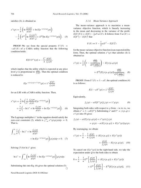
x ∗ (p) = 1 a<br />
− 1 a<br />
(<br />
ln f p(p)<br />
)<br />
g(p) + ln E[e−ay(p,q) |p]<br />
(E Q [<br />
ln f p(p)<br />
g(p)<br />
]<br />
+ E Q [ln E[e −ay(p,q) |p]]<br />
)<br />
. (5)<br />
PROOF: We see from the special property U ′ (Y ) =<br />
−aU(Y ) of a CARA utility function that the following<br />
condition holds:<br />
E[U(Y ∗ )|p] =− λ∗<br />
a<br />
g(p)<br />
f p (p) ,<br />
which implies that the utility which is expected at any price<br />
level p is proportional to g(p)<br />
f p<br />
. Then the optimal condition<br />
(p)<br />
is reduced to<br />
E[e −a(y(p,q)+x∗ (p)) |p] =λ ∗ g(p)<br />
f p (p)<br />
for an LSE <strong>with</strong> a CARA utility function. Then,<br />
x ∗ (p) = 1 ( )<br />
1<br />
a ln f p (p)<br />
λ ∗ g(p) E[e−ay(p,q) |p]<br />
= 1 (<br />
− ln λ ∗ + ln f )<br />
p(p)<br />
a<br />
g(p) + ln E[e−ay(p,q) |p] . (6)<br />
The Lagrange multiplier λ ∗ in the equation should satisfy the<br />
zero-cost constraint (2), which is ∫ ∞<br />
−∞ x∗ (p)g(p)dp = 0.<br />
That is,<br />
∫ ∞<br />
−∞<br />
(<br />
1<br />
− ln λ ∗ + ln f p(p)<br />
a<br />
g(p)<br />
)<br />
+ ln E[e −ay(p,q) |p] g(p)dp = 0. (7)<br />
Solving (7) for ln λ ∗ gives<br />
ln λ ∗ =<br />
∫ ∞<br />
−∞<br />
(<br />
ln f )<br />
p(p)<br />
g(p) + ln E[e−ay(p,q) |p] g(p)dp.<br />
Substituting this into Eq. (6) gives the optimal solution (5).<br />
□<br />
3.1.4. Mean-Variance Approach<br />
The mean-variance approach is to maximize a meanvariance<br />
objective function, which is linearly increasing<br />
in the mean and decreasing in the variance of the profit:<br />
E[U(Y)]=E[Y ]− 1 aV ar(Y). It follows from Var(Y)=<br />
2<br />
E[Y 2 ]−E[Y ] 2 that<br />
U(Y) ≡ Y − 1 2 a(Y 2 − E[Y ] 2 )<br />
for the mean-variance objective function in an expected utility<br />
form. Then, the optimal solution x ∗ (p) that satisfies (4) is<br />
obtained as<br />
(<br />
x ∗ (p) = 1 g(p) )<br />
f p (p)<br />
1 −<br />
a E Q[ g(p)<br />
] − E[y(p, q)|p]<br />
f p (p)<br />
+ E Q [E[y(p, q)|p]]<br />
g(p)<br />
f p (p)<br />
E Q[ g(p)<br />
f p (p)<br />
]. (8)<br />
PROOF: From U ′ (Y ) = 1 − aY, the optimal condition (4)<br />
is as follows:<br />
Equivalently,<br />
E[1 − aY ∗ |p] =λ ∗ g(p)<br />
f p (p) .<br />
f p (p) − aE[Y ∗ |p]f p (p) = λ ∗ g(p). (9)<br />
Integrating both sides <strong>with</strong> respect to p from −∞ to ∞, we<br />
obtain λ ∗ = 1−aE[Y ∗ ]. Substituting λ ∗ and Y ∗ = y(p, q)+<br />
x ∗ (p) into (9) gives<br />
f p (p) − a(E[y(p, q)|p]+x ∗ (p))f p (p)<br />
= g(p) − a(E[y(p, q)]+E[x ∗ (p)])g(p).<br />
By rearranging, we obtain<br />
x ∗ (p) = 1 a − 1 a<br />
g(p)<br />
f p (p) + (E[y(p, q)]+E[x∗ (p)])<br />
× g(p) − E[y(p, q)|p]. (10)<br />
f p (p)<br />
To cancel out E[x ∗ (p)] in the right-hand side, we take the<br />
expectation under Q to the both sides to obtain<br />
0 = 1 a − 1 [ ] g(p)<br />
a EQ + (E[y(p, q)]+E[x ∗ (p)])<br />
f p (p)<br />
× E Q [ g(p)<br />
f p (p)<br />
]<br />
− E Q [E[y(p, q)|p]], (11)<br />
Naval Research Logistics DOI 10.1002/nav


