Vector Space Semantic Parsing: A Framework for Compositional ...
Vector Space Semantic Parsing: A Framework for Compositional ...
Vector Space Semantic Parsing: A Framework for Compositional ...

Create successful ePaper yourself
Turn your PDF publications into a flip-book with our unique Google optimized e-Paper software.
ACL 2013<br />
51st Annual Meeting of the<br />
Association <strong>for</strong> Computational Linguistics<br />
Proceedings of the Workshop on Continuous <strong>Vector</strong> <strong>Space</strong><br />
Models and their <strong>Compositional</strong>ity<br />
August 9, 2013<br />
Sofia, Bulgaria
Production and Manufacturing by<br />
Omnipress, Inc.<br />
2600 Anderson Street<br />
Madison, WI 53704 USA<br />
c○2013 The Association <strong>for</strong> Computational Linguistics<br />
Order copies of this and other ACL proceedings from:<br />
Association <strong>for</strong> Computational Linguistics (ACL)<br />
209 N. Eighth Street<br />
Stroudsburg, PA 18360<br />
USA<br />
Tel: +1-570-476-8006<br />
Fax: +1-570-476-0860<br />
acl@aclweb.org<br />
ISBN: 978-1-937284-67-1<br />
ii
Introduction<br />
In recent years, there has been a growing interest in algorithms that learn a continuous representation<br />
<strong>for</strong> words, phrases, or documents. For instance, one can see latent semantic analysis (Landauer and<br />
Dumais, 1997) and latent Dirichlet allocation (Blei et al. 2003) as a mapping of documents or words into<br />
a continuous lower dimensional topic-space. Another example, continuous word vector-space models<br />
(Sahlgren 2006, Reisinger 2012, Turian et al., 2010, Huang et al., 2012) represent word meanings with<br />
vectors that capture semantic and syntactic in<strong>for</strong>mation. These representations can be used to induce<br />
similarity measures by computing distances between the vectors, leading to many useful applications,<br />
such as in<strong>for</strong>mation retrieval (Schuetze 1992, Manning et al., 2008), search query expansions (Jones et<br />
al., 2006), document classification (Sebastiani, 2002) and question answering (Tellex et al., 2003).<br />
On the fundamental task of language modeling, many hard clustering approaches have been proposed<br />
such as Brown clustering (Brown et al.,1992) or exchange clustering (Martin et al.,1998). These<br />
algorithms can provide desparsification and can be seen as examples of unsupervised pre-training.<br />
However, they have not been shown to consistently outper<strong>for</strong>m models based on Kneser-Ney smoothed<br />
language models which have at their core discrete n-gram representations. On the contrary, one<br />
influential proposal that uses the idea of continuous vector spaces <strong>for</strong> language modeling is that of neural<br />
language models (Bengio et al., 2003, Mikolov 2012). In these approaches, n-gram probabilities are<br />
estimated using a continuous representation of words in lieu of standard discrete representations, using<br />
a neural network that per<strong>for</strong>ms both the projection and the probability estimate. They report state of the<br />
art per<strong>for</strong>mance on several well studied language modeling datasets.<br />
Other neural network based models that use continuous vector representations achieve state of the art<br />
per<strong>for</strong>mance in speech recognition applications (Schwenk, 2007, Dahl et al. 2011), multitask learning,<br />
NER and POS tagging (Collobert et al., 2011) or sentiment analysis (Socher et al. 2011). Moreover, in<br />
(Le et al., 2012), a continuous space translation model was introduced and its use in a large scale machine<br />
translation system yielded promising results in the last WMT evaluation.<br />
Despite the success of single word vector space models, they are severely limited since they do not<br />
capture compositionality, the important quality of natural language that allows speakers to determine<br />
the meaning of a longer expression based on the meanings of its words and the rules used to combine<br />
them (Frege, 1892). This prevents them from gaining a deeper understanding of the semantics of longer<br />
phrases or sentences. Recently, there has been much progress in capturing compositionality in vector<br />
spaces, e.g., (Pado and Lapata 2007; Erk and Pado 2008; Mitchell and Lapata, 2010; Baroni and<br />
Zamparelli, 2010; Zanzotto et al., 2010; Yessenalina and Cardie, 2011; Grefenstette and Sadrzadeh<br />
2011). The work of Socher et al. 2012 compares several of these approaches on supervised tasks and <strong>for</strong><br />
phrases of arbitrary type and length.<br />
Another different trend of research belongs to the family of spectral methods. The motivation in that<br />
context is that working in a continuous space allows <strong>for</strong> the design of algorithms that are not plagued<br />
with the local minima issues that discrete latent space models (e.g. HMM trained with EM) tend to<br />
suffer from (Hsu et al. 2008). In fact, this motivation strikes with the conventional justification behind<br />
vector space models from the neural network literature, which are usually motivated as a way of tackling<br />
data sparsity issues. This apparent dichotomy is interesting and has not been investigated yet. Finally,<br />
spectral methods have recently been developed <strong>for</strong> word representation learning (Dhillon et al. 2011),<br />
dependency parsing (Dhillon et al. 2012) and probabilistic context-free grammars (Cohen et al. 2012).<br />
In this workshop, we bring together researchers who are interested in how to learn continuous vector<br />
space models, their compositionality and how to use this new kind of representation in NLP applications.<br />
The goal is to review the recent progress and propositions, to discuss the challenges, to identify promising<br />
future research directions and the next challenges <strong>for</strong> the NLP community.<br />
iii
Organizers:<br />
Alexandre Allauzen, LIMSI-CNRS/Université Paris-Sud<br />
Hugo Larochelle, Université de de Sherbrooke<br />
Richard Socher, Stan<strong>for</strong>d University<br />
Christopher Manning, Stan<strong>for</strong>d University<br />
Program Committee:<br />
Yoshua Bengio, Université de Montréal<br />
Antoine Bordes, Université Technologique de Compiègne<br />
Léon Bottou, Microsoft Research<br />
Xavier Carreras, Universitat Politècnica de Catalunya<br />
Shay Cohen, Columbia University<br />
Michael Collins, Columbia University<br />
Ronan Collobert, IDIAP Research Institute<br />
Kevin Duh, Nara Institute of Science and Technology<br />
Dean Foster, University of Pennsylvania<br />
Percy Liang, Stan<strong>for</strong>d University<br />
Andriy Mnih, Gatsby Computational Neuroscience Unit<br />
John Platt, Microsoft Research<br />
Holger Schwenk, Université du Maine<br />
Jason Weston, Google<br />
Guillaume Wisniewski, LIMSI-CNRS/Université<br />
Invited Speaker:<br />
Xavier Carreras, Universitat Politècnica de Catalunya<br />
Mirella Lapata, University of Edinburgh<br />
v
Table of Contents<br />
<strong>Vector</strong> <strong>Space</strong> <strong>Semantic</strong> <strong>Parsing</strong>: A <strong>Framework</strong> <strong>for</strong> <strong>Compositional</strong> <strong>Vector</strong> <strong>Space</strong> Models<br />
Jayant Krishnamurthy and Tom Mitchell . . . . . . . . . . . . . . . . . . . . . . . . . . . . . . . . . . . . . . . . . . . . . . . . . . . 1<br />
Learning from errors: Using vector-based compositional semantics <strong>for</strong> parse reranking<br />
Phong Le, Willem Zuidema and Remko Scha . . . . . . . . . . . . . . . . . . . . . . . . . . . . . . . . . . . . . . . . . . . . . . 11<br />
A Structured Distributional <strong>Semantic</strong> Model : Integrating Structure with <strong>Semantic</strong>s<br />
Kartik Goyal, Sujay Kumar Jauhar, Huiying Li, Mrinmaya Sachan, Shashank Srivastava and Eduard<br />
Hovy . . . . . . . . . . . . . . . . . . . . . . . . . . . . . . . . . . . . . . . . . . . . . . . . . . . . . . . . . . . . . . . . . . . . . . . . . . . . . . . . . . . . . . . 20<br />
Letter N-Gram-based Input Encoding <strong>for</strong> Continuous <strong>Space</strong> Language Models<br />
Henning Sperr, Jan Niehues and Alex Waibel . . . . . . . . . . . . . . . . . . . . . . . . . . . . . . . . . . . . . . . . . . . . . . 30<br />
Transducing Sentences to Syntactic Feature <strong>Vector</strong>s: an Alternative Way to "Parse"?<br />
Fabio Massimo Zanzotto and Lorenzo Dell’Arciprete. . . . . . . . . . . . . . . . . . . . . . . . . . . . . . . . . . . . . . .40<br />
General estimation and evaluation of compositional distributional semantic models<br />
Georgiana Dinu, Nghia The Pham and Marco Baroni . . . . . . . . . . . . . . . . . . . . . . . . . . . . . . . . . . . . . . . 50<br />
Applicative structure in vector space models<br />
Marton Makrai, David Mark Nemeskey and Andras Kornai . . . . . . . . . . . . . . . . . . . . . . . . . . . . . . . . . 59<br />
Determining <strong>Compositional</strong>ity of Expresssions Using Various Word <strong>Space</strong> Models and Methods<br />
Lubomír Krčmář, Karel Ježek and Pavel Pecina . . . . . . . . . . . . . . . . . . . . . . . . . . . . . . . . . . . . . . . . . . . . 64<br />
“Not not bad” is not “bad”: A distributional account of negation<br />
Karl Moritz Hermann, Edward Grefenstette and Phil Blunsom . . . . . . . . . . . . . . . . . . . . . . . . . . . . . . 74<br />
Towards Dynamic Word Sense Discrimination with Random Indexing<br />
Hans Moen, Erwin Marsi and Björn Gambäck . . . . . . . . . . . . . . . . . . . . . . . . . . . . . . . . . . . . . . . . . . . . . 83<br />
A Generative Model of <strong>Vector</strong> <strong>Space</strong> <strong>Semantic</strong>s<br />
Jacob Andreas and Zoubin Ghahramani . . . . . . . . . . . . . . . . . . . . . . . . . . . . . . . . . . . . . . . . . . . . . . . . . . . 91<br />
Aggregating Continuous Word Embeddings <strong>for</strong> In<strong>for</strong>mation Retrieval<br />
Stephane Clinchant and Florent Perronnin. . . . . . . . . . . . . . . . . . . . . . . . . . . . . . . . . . . . . . . . . . . . . . . .100<br />
Answer Extraction by Recursive Parse Tree Descent<br />
Christopher Malon and Bing Bai . . . . . . . . . . . . . . . . . . . . . . . . . . . . . . . . . . . . . . . . . . . . . . . . . . . . . . . . 110<br />
Recurrent Convolutional Neural Networks <strong>for</strong> Discourse <strong>Compositional</strong>ity<br />
Nal Kalchbrenner and Phil Blunsom . . . . . . . . . . . . . . . . . . . . . . . . . . . . . . . . . . . . . . . . . . . . . . . . . . . . . 119<br />
vii
Conference Program<br />
9:00 Opening<br />
(9:00) Oral session 1<br />
9:05 INVITED TALK: Structured Prediction with Low-Rank Bilinear Models by Xavier<br />
Carreras<br />
10:00 <strong>Vector</strong> <strong>Space</strong> <strong>Semantic</strong> <strong>Parsing</strong>: A <strong>Framework</strong> <strong>for</strong> <strong>Compositional</strong> <strong>Vector</strong> <strong>Space</strong><br />
Models<br />
Jayant Krishnamurthy and Tom Mitchell<br />
10:20 Learning from errors: Using vector-based compositional semantics <strong>for</strong> parse<br />
reranking<br />
Phong Le, Willem Zuidema and Remko Scha<br />
10:40 Coffee Break<br />
(11:00) Poster session<br />
A Structured Distributional <strong>Semantic</strong> Model : Integrating Structure with <strong>Semantic</strong>s<br />
Kartik Goyal, Sujay Kumar Jauhar, Huiying Li, Mrinmaya Sachan, Shashank Srivastava<br />
and Eduard Hovy<br />
Letter N-Gram-based Input Encoding <strong>for</strong> Continuous <strong>Space</strong> Language Models<br />
Henning Sperr, Jan Niehues and Alex Waibel<br />
Transducing Sentences to Syntactic Feature <strong>Vector</strong>s: an Alternative Way to "Parse"?<br />
Fabio Massimo Zanzotto and Lorenzo Dell’Arciprete<br />
General estimation and evaluation of compositional distributional semantic models<br />
Georgiana Dinu, Nghia The Pham and Marco Baroni<br />
Applicative structure in vector space models<br />
Marton Makrai, David Mark Nemeskey and Andras Kornai<br />
Determining <strong>Compositional</strong>ity of Expresssions Using Various Word <strong>Space</strong> Models<br />
and Methods<br />
Lubomír Krčmář, Karel Ježek and Pavel Pecina<br />
“Not not bad” is not “bad”: A distributional account of negation<br />
Karl Moritz Hermann, Edward Grefenstette and Phil Blunsom<br />
ix
Poster session (continued)<br />
12:30 Lunch Break<br />
Towards Dynamic Word Sense Discrimination with Random Indexing<br />
Hans Moen, Erwin Marsi and Björn Gambäck<br />
(14:00) Oral session 2<br />
14:00 INVITED TALK: Learning to Ground Meaning in the Visual World by Mirella Lapata<br />
15:00 A Generative Model of <strong>Vector</strong> <strong>Space</strong> <strong>Semantic</strong>s<br />
Jacob Andreas and Zoubin Ghahramani<br />
15:20 Aggregating Continuous Word Embeddings <strong>for</strong> In<strong>for</strong>mation Retrieval<br />
Stephane Clinchant and Florent Perronnin<br />
15:40 Coffee Break<br />
16:00 Answer Extraction by Recursive Parse Tree Descent<br />
Christopher Malon and Bing Bai<br />
16:20 Recurrent Convolutional Neural Networks <strong>for</strong> Discourse <strong>Compositional</strong>ity<br />
Nal Kalchbrenner and Phil Blunsom<br />
(16:40) Panel Discussion<br />
x
<strong>Vector</strong> <strong>Space</strong> <strong>Semantic</strong> <strong>Parsing</strong>: A <strong>Framework</strong> <strong>for</strong><br />
<strong>Compositional</strong> <strong>Vector</strong> <strong>Space</strong> Models<br />
Jayant Krishnamurthy<br />
Carnegie Mellon University<br />
5000 Forbes Avenue<br />
Pittsburgh, PA 15213<br />
jayantk@cs.cmu.edu<br />
Tom M. Mitchell<br />
Carnegie Mellon University<br />
5000 Forbes Avenue<br />
Pittsburgh, PA 15213<br />
tom.mitchell@cmu.edu<br />
Abstract<br />
We present vector space semantic parsing<br />
(VSSP), a framework <strong>for</strong> learning compositional<br />
models of vector space semantics.<br />
Our framework uses Combinatory Categorial<br />
Grammar (CCG) to define a correspondence<br />
between syntactic categories<br />
and semantic representations, which are<br />
vectors and functions on vectors. The<br />
complete correspondence is a direct consequence<br />
of minimal assumptions about<br />
the semantic representations of basic syntactic<br />
categories (e.g., nouns are vectors),<br />
and CCG’s tight coupling of syntax and<br />
semantics. Furthermore, this correspondence<br />
permits nonuni<strong>for</strong>m semantic representations<br />
and more expressive composition<br />
operations than previous work. VSSP<br />
builds a CCG semantic parser respecting<br />
this correspondence; this semantic parser<br />
parses text into lambda calculus <strong>for</strong>mulas<br />
that evaluate to vector space representations.<br />
In these <strong>for</strong>mulas, the meanings of<br />
words are represented by parameters that<br />
can be trained in a task-specific fashion.<br />
We present experiments using noun-verbnoun<br />
and adverb-adjective-noun phrases<br />
which demonstrate that VSSP can learn<br />
composition operations that RNN (Socher<br />
et al., 2011) and MV-RNN (Socher et al.,<br />
2012) cannot.<br />
1 Introduction<br />
<strong>Vector</strong> space models represent the semantics of<br />
natural language using vectors and operations on<br />
vectors (Turney and Pantel, 2010). These models<br />
are most commonly used <strong>for</strong> individual words and<br />
short phrases, where vectors are created using distributional<br />
in<strong>for</strong>mation from a corpus. Such models<br />
achieve impressive per<strong>for</strong>mance on standardized<br />
tests (Turney, 2006; Rapp, 2003), correlate<br />
well with human similarity judgments (Griffiths et<br />
al., 2007), and have been successfully applied to a<br />
number of natural language tasks (Collobert et al.,<br />
2011).<br />
While vector space representations <strong>for</strong> individual<br />
words are well-understood, there remains<br />
much uncertainty about how to compose vector<br />
space representations <strong>for</strong> phrases out of their component<br />
words. Recent work in this area raises<br />
many important theoretical questions. For example,<br />
should all syntactic categories of words be<br />
represented as vectors, or are some categories,<br />
such as adjectives, different? Using distinct semantic<br />
representations <strong>for</strong> distinct syntactic categories<br />
has the advantage of representing the operational<br />
nature of modifier words, but the disadvantage<br />
of more complex parameter estimation (Baroni<br />
and Zamparelli, 2010). Also, does semantic<br />
composition factorize according to a constituency<br />
parse tree (Socher et al., 2011; Socher et al.,<br />
2012)? A binarized constituency parse cannot directly<br />
represent many intuitive intra-sentence dependencies,<br />
such as the dependence between a<br />
verb’s subject and its object. What is needed to<br />
resolve these questions is a comprehensive theoretical<br />
framework <strong>for</strong> compositional vector space<br />
models.<br />
In this paper, we observe that we already have<br />
such a framework: Combinatory Categorial Grammar<br />
(CCG) (Steedman, 1996). CCG provides a<br />
tight mapping between syntactic categories and<br />
semantic types. If we assume that nouns, sentences,<br />
and other basic syntactic categories are<br />
represented by vectors, this mapping prescribes<br />
semantic types <strong>for</strong> all other syntactic categories. 1<br />
For example, we get that adjectives are functions<br />
from noun vectors to noun vectors, and that prepo-<br />
1 It is not necessary to assume that sentences are vectors.<br />
However, this assumption simplifies presentation and seems<br />
like a reasonable first step. CCG can be used similarly to<br />
explore alternative representations.<br />
1<br />
Proceedings of the Workshop on Continuous <strong>Vector</strong> <strong>Space</strong> Models and their <strong>Compositional</strong>ity, pages 1–10,<br />
Sofia, Bulgaria, August 9 2013. c○2013 Association <strong>for</strong> Computational Linguistics
Input:<br />
Log. Form:<br />
“red ball” → semantic → A<br />
parsing red v ball → evaluation → „ «<br />
◦<br />
◦<br />
↑<br />
↑<br />
„<br />
◦ ◦<br />
◦ ◦<br />
Lexicon: red:= λx.A redx<br />
Params.: A<br />
ball:= v red =<br />
ball<br />
„ «<br />
◦<br />
v ball =<br />
◦<br />
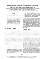
Figure 1: Overview of vector space semantic parsing<br />
(VSSP). A semantic parser first translates natural<br />
language into a logical <strong>for</strong>m, which is then<br />
evaluated to produce a vector.<br />
sitions are functions from a pair of noun vectors<br />
to a noun vector. These semantic type specifications<br />
permit a variety of different composition operations,<br />
many of which cannot be represented in<br />
previously-proposed frameworks. <strong>Parsing</strong> in CCG<br />
applies these functions to each other, naturally deriving<br />
a vector space representation <strong>for</strong> an entire<br />
phrase.<br />
The CCG framework provides function type<br />
specifications <strong>for</strong> each word’s semantics, given its<br />
syntactic category. Instantiating this framework<br />
amounts to selecting particular functions <strong>for</strong> each<br />
word. <strong>Vector</strong> space semantic parsing (VSSP) produces<br />
these per-word functions in a two-step process.<br />
The first step chooses a parametric functional<br />
<strong>for</strong>m <strong>for</strong> each syntactic category, which contains<br />
as-yet unknown per-word and global parameters.<br />
The second step estimates these parameters<br />
using a concrete task of interest, such as predicting<br />
the corpus statistics of adjective-noun compounds.<br />
We present a stochastic gradient algorithm <strong>for</strong> this<br />
step which resembles training a neural network<br />
with backpropagation. These parameters may also<br />
be estimated in an unsupervised fashion, <strong>for</strong> example,<br />
using distributional statistics.<br />
Figure 1 presents an overview of VSSP. The<br />
input to VSSP is a natural language phrase and<br />
a lexicon, which contains the parametrized functional<br />
<strong>for</strong>ms <strong>for</strong> each word. These per-word representations<br />
are combined by CCG semantic parsing<br />
to produce a logical <strong>for</strong>m, which is a symbolic<br />
mathematical <strong>for</strong>mula <strong>for</strong> producing the vector<br />
<strong>for</strong> a phrase – <strong>for</strong> example, A red v ball is a <strong>for</strong>mula<br />
that per<strong>for</strong>ms matrix-vector multiplication.<br />
This <strong>for</strong>mula is evaluated using learned per-word<br />
and global parameters (values <strong>for</strong> A red and v ball )<br />
to produce the language’s vector space representation.<br />
The contributions of this paper are threefold.<br />
«<br />
First, we demonstrate how CCG provides a theoretical<br />
basis <strong>for</strong> vector space models. Second,<br />
we describe VSSP, which is a method <strong>for</strong> concretely<br />
instantiating this theoretical framework.<br />
Finally, we per<strong>for</strong>m experiments comparing VSSP<br />
against other compositional vector space models.<br />
We per<strong>for</strong>m two case studies of composition<br />
using noun-verb-noun and adverb-adjective-noun<br />
phrases, finding that VSSP can learn composition<br />
operations that existing models cannot. We also<br />
find that VSSP produces intuitively reasonable parameters.<br />
2 Combinatory Categorial Grammar <strong>for</strong><br />
<strong>Vector</strong> <strong>Space</strong> Models<br />
Combinatory Categorial Grammar (CCG) (Steedman,<br />
1996) is a lexicalized grammar <strong>for</strong>malism<br />
that has been used <strong>for</strong> both broad coverage syntactic<br />
parsing and semantic parsing. Like other lexicalized<br />
<strong>for</strong>malisms, CCG has a rich set of syntactic<br />
categories, which are combined using a small<br />
set of parsing operations. These syntactic categories<br />
are tightly coupled to semantic representations,<br />
and parsing in CCG simultaneously derives<br />
both a syntactic parse tree and a semantic<br />
representation <strong>for</strong> each node in the parse tree.<br />
This coupling between syntax and semantics motivates<br />
CCG’s use in semantic parsing (Zettlemoyer<br />
and Collins, 2005), and provides a framework <strong>for</strong><br />
building compositional vector space models.<br />
2.1 Syntax<br />
The intuition embodied in CCG is that, syntactically,<br />
words and phrases behave like functions.<br />
For example, an adjective like “red” can combine<br />
with a noun like “ball” to produce another<br />
noun, “red ball.” There<strong>for</strong>e, adjectives are naturally<br />
viewed as functions that apply to nouns and<br />
return nouns. CCG generalizes this idea by defining<br />
most parts of speech in terms of such functions.<br />
Parts of speech in CCG are called syntactic categories.<br />
CCG has two kinds of syntactic categories:<br />
atomic categories and functional categories.<br />
Atomic categories are used to represent<br />
phrases that do not accept arguments. These categories<br />
include N <strong>for</strong> noun, NP <strong>for</strong> noun phrase, S<br />
<strong>for</strong> sentence, and P P <strong>for</strong> prepositional phrase. All<br />
other parts of speech are represented using functional<br />
categories. Functional categories are written<br />
as X/Y or X\Y , where both X and Y are syn-<br />
2
Part of speech Syntactic category Example usage <strong>Semantic</strong> type Example log. <strong>for</strong>m<br />
Noun N person : N R d v person<br />
Adjective N/N x good person : N 〈R d , R d 〉 λx.A good x<br />
Determiner NP/N x the person : NP 〈R d , R d 〉 λx.x<br />
Intrans. Verb S\NP x the person ran : S 〈R d , R d 〉 λx.A ranx + b ran<br />
Trans. Verb S\NP y/NP x the person ran home : S 〈R d , 〈R d , R d 〉〉 λx.λy.(T ranx)y<br />
Adverb (S\NP )\(S\NP ) ran lazily : S\NP 〈〈R d , R d 〉, 〈R d , R d 〉〉 [λy.Ay → λy.(T lazy A)y]<br />
(S\NP )/(S\NP ) lazily ran : S\NP 〈〈R d , R d 〉, 〈R d , R d 〉〉 [λy.Ay → λy.(T lazy A)y]<br />
(N/N)/(N/N) very good person : N 〈〈R d , R d 〉, 〈R d , R d 〉〉 [λy.Ay → λy.(T veryA)y]<br />
Preposition (N\N y)/N x person in France : N 〈R d , 〈R d , R d 〉〉 λx.λy.(T inx)y<br />
(S\NP y)\(S\NP ) f /NP x ran in France : S\NP 〈R d , 〈〈R d , R d 〉, 〈R d , R d 〉〉〉 λx.λf.λy.(T inx)(f(y))<br />
Table 1: Common syntactic categories in CCG, paired with their semantic types and example logical<br />
<strong>for</strong>ms. The example usage column shows phrases paired with the syntactic category that results from<br />
using the exemplified syntactic category <strong>for</strong> the bolded word. For ease of reference, each argument to<br />
a syntactic category on the left is subscripted with its corresponding semantic variable in the example<br />
logical <strong>for</strong>m on the right. The variables x, y, b, v denote vectors, f denotes a function, A denotes a<br />
matrix, and T denotes a tensor. Subscripted variables (A red ) denote parameters. Functions in logical<br />
<strong>for</strong>ms are specified using lambda calculus; <strong>for</strong> example λx.Ax is the function that accepts a (vector)<br />
argument x and returns the vector Ax. The notation [f → g] denotes the higher-order function that,<br />
given input function f, outputs function g.<br />
tactic categories. These categories represent functions<br />
that accept an argument of category Y and<br />
return a phrase of category X. The direction of<br />
the slash defines the expected location of the argument:<br />
X/Y expects an argument on the right, and<br />
X\Y expects an argument on the left. 2 For example,<br />
adjectives are represented by the category<br />
N/N – a function that accepts a noun on the right<br />
and returns a noun.<br />
The left part of Table 1 shows examples of<br />
common syntactic categories, along with example<br />
uses. Note that some intuitive parts of speech,<br />
such as prepositions, are represented by multiple<br />
syntactic categories. Each of these categories captures<br />
a different use of a preposition, in this case<br />
the noun-modifying and verb-modifying uses.<br />
2.2 <strong>Semantic</strong>s<br />
<strong>Semantic</strong>s in CCG are given by first associating a<br />
semantic type with each syntactic category. Each<br />
word in a syntactic category is then assigned a<br />
semantic representation of the corresponding semantic<br />
type. These semantic representations are<br />
known as logical <strong>for</strong>ms. In our case, a logical <strong>for</strong>m<br />
is a fragment of a <strong>for</strong>mula <strong>for</strong> computing a vector<br />
space representation, containing word-specific parameters<br />
and specifying composition operations.<br />
In order to construct a vector space model, we<br />
associate all of the atomic syntactic categories,<br />
2 As a memory aid, note that the top of the slash points in<br />
the direction of the expected argument.<br />
N, NP , S, and P P , with the type R d . Then,<br />
the logical <strong>for</strong>m <strong>for</strong> a noun like “ball” is a vector<br />
v ball ∈ R d . The functional categories X/Y<br />
and X\Y are associated with functions from the<br />
semantic type of X to the semantic type of Y . For<br />
example, the semantic type of N/N is 〈R d , R d 〉,<br />
representing the set of functions from R d to R d . 3<br />
This semantic type captures the same intuition as<br />
adjective-noun composition models: semantically,<br />
adjectives are functions from noun vectors to noun<br />
vectors.<br />
The right portion of Table 1 shows semantic<br />
types <strong>for</strong> several syntactic categories, along with<br />
example logical <strong>for</strong>ms. All of these mappings<br />
are a direct consequence of the assumption that<br />
all atomic categories are semantically represented<br />
by vectors. Interestingly, many of these semantic<br />
types contain functions that cannot be represented<br />
in other frameworks. For example, adverbs have<br />
type 〈〈R d , R d 〉, 〈R d , R d 〉〉, representing functions<br />
that accept an adjective argument and return an<br />
adjective. In Table 1, the example logical <strong>for</strong>m<br />
applies a 4-mode tensor to the adjective’s matrix.<br />
Another powerful semantic type is 〈R d , 〈R d , R d 〉〉,<br />
which corresponds to transitive verbs and prepo-<br />
3 The notation 〈A, B〉 represents the set of functions<br />
whose domain is A and whose range is B. Somewhat confusingly,<br />
the bracketing in this notation is backward relative to<br />
the syntactic categories – the syntactic category (N\N)/N<br />
has semantic type 〈R d , 〈R d , R d 〉〉, where the inner 〈R d , R d 〉<br />
corresponds to the left (N\N).<br />
3
the<br />
NP/N<br />
λx.x<br />
red<br />
N/N<br />
λx.A red x<br />
ball<br />
N<br />
v ball<br />
on<br />
(NP \NP )/NP<br />
λx.λy.A onx + B ony<br />
the<br />
NP/N<br />
λx.x<br />
table<br />
N<br />
v table<br />
N : A red v ball<br />
NP : A red v ball<br />
NP : v table<br />
NP \NP : λy.A onv table + B ony<br />
NP : A onv table + B onA red v ball<br />
Figure 2: Syntactic CCG parse and corresponding vector space semantic derivation.<br />
sitions. This type represents functions from two<br />
argument vectors to an output vector, which have<br />
been curried to accept one argument vector at a<br />
time. The example logical <strong>for</strong>m <strong>for</strong> this type uses<br />
a 3-mode tensor to capture interactions between<br />
the two arguments.<br />
Note that this semantic correspondence permits<br />
a wide range of logical <strong>for</strong>ms <strong>for</strong> each syntactic<br />
category. Each logical <strong>for</strong>m can have an arbitrary<br />
functional <strong>for</strong>m, as long as it has the correct semantic<br />
type. This flexibility permits experimentation<br />
with different composition operations. For example,<br />
adjectives can be represented nonlinearly<br />
by using a logical <strong>for</strong>m such as λx. tanh(Ax). Or,<br />
adjectives can be represented nonparametrically<br />
by using kernel regression to learn the appropriate<br />
function from vectors to vectors. We can also introduce<br />
simplifying assumptions, as demonstrated<br />
by the last entry in Table 1. CCG treats prepositions<br />
as modifying intransitive verbs (the category<br />
S\N). In the example logical <strong>for</strong>m, the verb’s<br />
semantics are represented by the function f, the<br />
verb’s subject noun is represented by y, and f(y)<br />
represents the sentence vector created by composing<br />
the verb with its argument. By only operating<br />
on f(y), this logical <strong>for</strong>m assumes that the action<br />
of a preposition is conditionally independent of the<br />
verb f and noun y, given the sentence f(y).<br />
2.3 Lexicon<br />
The main input to a CCG parser is a lexicon, which<br />
is a mapping from words to syntactic categories<br />
and logical <strong>for</strong>ms. A lexicon contains entries such<br />
as:<br />
ball := N : v ball<br />
red := N/N : λx.A red x<br />
red := N : v red<br />
flies := ((S\NP )/NP ) : λx.λy.(T flies x)y<br />
Each entry of the lexicon associates a word<br />
(ball) with a syntactic category (N) and a logical<br />
<strong>for</strong>m (v ball ) giving its vector space representation.<br />
Note that a word may appear multiple times in the<br />
lexicon with distinct syntactic categories and logical<br />
<strong>for</strong>ms. Such repeated entries capture words<br />
with multiple possible uses; parsing must determine<br />
the correct use in the context of a sentence.<br />
2.4 <strong>Parsing</strong><br />
<strong>Parsing</strong> in CCG has two stages. First, a category<br />
<strong>for</strong> each word in the input is retrieved from the lexicon.<br />
Second, adjacent categories are iteratively<br />
combined by applying one of a small number of<br />
combinators. The most common combinator is<br />
function application:<br />
X/Y : f Y : g =⇒ X : f(g)<br />
Y : g X\Y : f =⇒ X : f(g)<br />
The function application rule states that a category<br />
of the <strong>for</strong>m X/Y behaves like a function that<br />
accepts an input category Y and returns category<br />
X. The rule also derives a logical <strong>for</strong>m <strong>for</strong> the result<br />
by applying the function f (the logical <strong>for</strong>m<br />
<strong>for</strong> X/Y ) to g (the logical <strong>for</strong>m <strong>for</strong> Y ). Figure 2<br />
shows how repeatedly applying this rule produces<br />
a syntactic parse tree and logical <strong>for</strong>m <strong>for</strong> a phrase.<br />
The top row of the parse represents retrieving a<br />
lexicon entry <strong>for</strong> each word in the input. Each<br />
following line represents a use of the function application<br />
combinator to syntactically and semantically<br />
combine a pair of adjacent categories. The<br />
order of these operations is ambiguous, and different<br />
orderings may result in different parses – a<br />
CCG parser’s job is to find a correct ordering. The<br />
result of parsing is a syntactic category <strong>for</strong> the entire<br />
phrase, coupled with a logical <strong>for</strong>m giving the<br />
phrase’s vector space representation.<br />
3 <strong>Vector</strong> <strong>Space</strong> <strong>Semantic</strong> <strong>Parsing</strong><br />
<strong>Vector</strong> space semantic parsing (VSSP) is an<br />
approach <strong>for</strong> constructing compositional vector<br />
space models based on the theoretical framework<br />
of the previous section. VSSP concretely instantiates<br />
CCG’s syntactic/semantic correspondence by<br />
adding appropriately-typed logical <strong>for</strong>ms to a syntactic<br />
CCG parser’s lexicon. <strong>Parsing</strong> a sentence<br />
with this lexicon and evaluating the resulting logi-<br />
4
<strong>Semantic</strong> type Example syntactic categories Logical <strong>for</strong>m template<br />
R d N, NP, P P, S v w<br />
〈R d , R d 〉 N/N, NP/N, S/S, S\NP λx.σ(A wx)<br />
〈R d , 〈R d , R d 〉〉 (S\NP )/NP , (NP \NP )/NP λx.λy.σ((T wx)y)<br />
〈〈R d , R d 〉, 〈R d , R d 〉〉 (N/N)/(N/N)<br />
[λy.σ(Ay) → λy.σ((T wA)y)]<br />
Table 2: Lexicon templates used in this paper to produce a CCG semantic parser. σ represents the<br />
sigmoid function, σ(x) =<br />
ex<br />
1+e<br />
. x<br />
cal <strong>for</strong>m produces the sentence’s vector space representation.<br />
While it is relatively easy to devise vector space<br />
representations <strong>for</strong> individual nouns, it is more<br />
challenging to do so <strong>for</strong> the fairly complex function<br />
types licensed by CCG. VSSP defines these<br />
functions in two phases. First, we create a lexicon<br />
mapping words to parametrized logical <strong>for</strong>ms.<br />
This lexicon specifies a functional <strong>for</strong>m <strong>for</strong> each<br />
word, but leaves free some per-word parameters.<br />
<strong>Parsing</strong> with this lexicon produces logical<br />
<strong>for</strong>ms that are essentially functions from these<br />
per-word parameters to vector space representations.<br />
Next, we train these parameters to produce<br />
good vector space representations in a taskspecific<br />
fashion. Training per<strong>for</strong>ms stochastic gradient<br />
descent, backpropagating gradient in<strong>for</strong>mation<br />
through the logical <strong>for</strong>ms.<br />
3.1 Producing the Parametrized Lexicon<br />
We create a lexicon using a set of manuallyconstructed<br />
templates that associate each syntactic<br />
category with a parametrized logical <strong>for</strong>m. Each<br />
template contains variables that are instantiated to<br />
define per-word parameters. The output of this<br />
step is a CCG lexicon which can be used in a<br />
broad coverage syntactic CCG parser (Clark and<br />
Curran, 2007) to produce logical <strong>for</strong>ms <strong>for</strong> input<br />
language. 4<br />
Table 2 shows some templates used to create<br />
logical <strong>for</strong>ms <strong>for</strong> syntactic categories. To reduce<br />
annotation ef<strong>for</strong>t, we define one template per semantic<br />
type, covering all syntactic categories with<br />
that type. These templates are instantiated by replacing<br />
the variable w in each logical <strong>for</strong>m with<br />
the current word. For example, instantiating the<br />
second template <strong>for</strong> “red” produces the logical<br />
<strong>for</strong>m λx.σ(A red x), where A red is a matrix of parameters.<br />
4 In order to use the lexicon in an existing parser, the generated<br />
syntactic categories must match the parser’s syntactic<br />
categories. Then, to produce a logical <strong>for</strong>m <strong>for</strong> a sentence,<br />
simply syntactically parse the sentence, generate logical<br />
<strong>for</strong>ms <strong>for</strong> each input word, and retrace the syntactic<br />
derivation while applying the corresponding semantic operations<br />
to the logical <strong>for</strong>ms.<br />
Note that Table 2 is a only starting point – devising<br />
appropriate functional <strong>for</strong>ms <strong>for</strong> each syntactic<br />
category is an empirical question that requires further<br />
research. We use these templates in our experiments<br />
(Section 4), suggesting that they are a<br />
reasonable first step. More complex data sets will<br />
require more complex logical <strong>for</strong>ms. For example,<br />
to use high-dimensional vectors, all matrices and<br />
tensors will have to be made low rank. Another<br />
possible improvement is to tie the parameters <strong>for</strong><br />
a single word across related syntactic categories<br />
(such as the transitive and intransitive <strong>for</strong>ms of a<br />
verb).<br />
3.2 Training the Logical Form Parameters<br />
The training problem in VSSP is to optimize the<br />
logical <strong>for</strong>m parameters to best per<strong>for</strong>m a given<br />
task. Our task <strong>for</strong>mulation subsumes both classification<br />
and regression: we assume the input is<br />
a logical <strong>for</strong>m, and the output is a vector. Given a<br />
data set of this <strong>for</strong>m, training can be per<strong>for</strong>med using<br />
stochastic gradient descent in a fashion similar<br />
to backpropagation in a neural network.<br />
The data set <strong>for</strong> training consists of tuples,<br />
{(l i , y i )} n i=1 , where l is a logical <strong>for</strong>m and y is a<br />
label vector representing the expected task output.<br />
Each logical <strong>for</strong>m l is treated as a function from<br />
parameter vectors θ to vectors in R d . For example,<br />
the logical <strong>for</strong>m A red v ball is a function from A red<br />
and v ball to a vector. We use θ to denote the set<br />
of all parameters; <strong>for</strong> example, θ = {A red , v ball }.<br />
We further assume a loss function L defined over<br />
pairs of label vectors. The training problem is<br />
there<strong>for</strong>e to minimize the objective:<br />
n∑<br />
O(θ) = L(y i , g(l i (θ)) + λ 2 ||θ||2<br />
i=1<br />
Above, g represents a global postprocessing function<br />
which is applied to the output of VSSP to<br />
make a task-specific prediction. This function may<br />
also be parametrized, but we suppress these parameters<br />
<strong>for</strong> simplicity. As a concrete example,<br />
consider a classification task (as in our evaluation).<br />
In this case, y represents a target distribution over<br />
labels, L is the KL divergence between the pre-<br />
5
dicted and target distributions, and g represents a<br />
softmax classifier.<br />
We optimize the objective O by running<br />
stochastic gradient descent. The gradients of the<br />
parameters θ can be computed by iteratively applying<br />
the chain rule to l, which procedurally<br />
resembles per<strong>for</strong>ming backpropagation in a neural<br />
network (Rumelhart et al., 1988; Goller and<br />
Küchler, 1996).<br />
4 Comparing Models of <strong>Semantic</strong><br />
Composition<br />
This section compares the expressive power of<br />
VSSP to previous work. An advantage of VSSP<br />
is its ability to assign complex logical <strong>for</strong>ms to<br />
categories like adverbs and transitive verbs. This<br />
section examines cases where such complex logical<br />
<strong>for</strong>ms are necessary, using synthetic data sets.<br />
Specifically, we create simple data sets mimicking<br />
expected <strong>for</strong>ms of composition in noun-verbnoun<br />
and adverb-adjective-noun phrases. VSSP<br />
is able to learn the correct composition operations<br />
<strong>for</strong> these data sets, but previously proposed models<br />
cannot.<br />
We compare VSSP against RNN (Socher et al.,<br />
2011) and MV-RNN (Socher et al., 2012), two<br />
recursive neural network models which factorize<br />
composition according to a binarized constituency<br />
parse tree. The RNN model represents the semantics<br />
of each parse tree node using a single vector,<br />
while the MV-RNN represents each node using<br />
both a matrix and a vector. These representations<br />
seem sufficient <strong>for</strong> adjectives and nouns, but it is<br />
unclear how they generalize to other natural language<br />
constructions.<br />
In these experiments, each model is used to map<br />
an input phrase to a vector, which is used to train a<br />
softmax classifier that predicts the task output. For<br />
VSSP, we use the lexicon templates from Table 2.<br />
All nouns are represented as two-dimensional vectors,<br />
and all matrices and tensors are full rank. The<br />
parameters of each model (i.e., the per-word vectors,<br />
matrices and tensors) and the softmax classifier<br />
are trained as described in Section 3.2.<br />
4.1 Propositional Logic<br />
The propositional logic experiment examines the<br />
impact of VSSP’s representation of transitive<br />
verbs. VSSP directly represents these verbs as<br />
two-argument functions, allowing it to learn operations<br />
with complex interactions between both<br />
false and false 0,1 false or false 0,1 false xor false 0,1<br />
true and false 0,1 true or false 1,0 true xor false 1,0<br />
false and true 0,1 false or true 1,0 false xor true 1,0<br />
true and true 1,0 true or true 1,0 true xor true 0,1<br />
Table 3: Data <strong>for</strong> propositional logic experiment.<br />
Composition Formula KL divergence<br />
RNN 0.44<br />
MV-RNN 0.12<br />
VSSP 0.01<br />
Table 4: Training error on the propositional logic<br />
data set. VSSP achieves zero error because its<br />
verb representation can learn arbitrary logical operations.<br />
arguments. In contrast, the RNN and MV-RNN<br />
models learn a set of global weights which are<br />
used to combine the verb with its arguments. The<br />
functional <strong>for</strong>ms of these models limit the kinds of<br />
interactions that can be captured by verbs.<br />
We evaluated the learnability of argument interactions<br />
using the simple data set shown in Table<br />
3. In this data set, the words “and,” “or,” and<br />
“xor” are treated as transitive verbs, while “true”<br />
and “false” are nouns. The goal is to predict the<br />
listed truth values, which are represented as twodimensional<br />
distributions over true and false.<br />
Table 4 shows the training error of each model<br />
on this data set, measured in terms of KL divergence<br />
between the model’s predictions and the<br />
true values. VSSP achieves essentially zero training<br />
error because its 3-mode tensor representation<br />
of transitive verbs is trivially able to learn<br />
arbitrary logical operations. RNN and MV-RNN<br />
can learn each logical operation independently, but<br />
cannot learn all three at the same time – this phenomenon<br />
occurs because XOR requires different<br />
global weight matrices than AND/OR. As a result,<br />
these models learn both AND and OR, but fail<br />
to learn XOR. This result suggests that much of<br />
the learning in these models occurs in the global<br />
weight matrices, while the verb representations<br />
can have only limited influence.<br />
Although this data set is synthetic, the interaction<br />
given by XOR seems necessary to represent<br />
real verbs. To learn AND and OR, the arguments<br />
need not interact – it is sufficient to detect a set<br />
of appropriate subject and object arguments, then<br />
threshold the number of such arguments. This<br />
in<strong>for</strong>mation is essentially type constraints <strong>for</strong> the<br />
subject and object of a verb. However, type constraints<br />
are insufficient <strong>for</strong> real verbs. For example,<br />
consider the verb “eats.” All animals eat and<br />
6
very big elephant 1,0 very big mouse 0.3,0.7<br />
pretty big elephant 0.9,0.1 pretty big mouse 0.2,0.8<br />
pretty small elephant 0.8,0.2 pretty small mouse 0.1,0.9<br />
very small elephant 0.7,0.3 very small mouse 0,1<br />
Table 5: Data <strong>for</strong> adverb-adjective-noun composition<br />
experiment. Higher first dimension values<br />
represent larger objects.<br />
Composition Model KL divergence<br />
RNN 0.10<br />
MV-RNN 0.10<br />
VSSP 0.00<br />
Table 6: Training error of each composition model<br />
on the adverb-adjective-noun experiment.<br />
can be eaten, but not all animals eat all other animals;<br />
whether or not “X eats Y ” is true depends<br />
on an interaction between X and Y .<br />
4.2 Adverb-Adjective-Noun Composition<br />
Adverbs can enhance or attenuate the properties<br />
of adjectives, which in turn can enhance or attenuate<br />
the properties of nouns. The adverb-adjectivenoun<br />
experiment compares each model’s ability<br />
to learn these effects using a synthetic object size<br />
data set, shown in Table 5. The task is to predict<br />
the size of each described object, which is represented<br />
as a two-dimensional distribution over big<br />
and small. The challenge of this data set is that<br />
an adverb’s impact on size depends on the adjective<br />
being modified – a very big elephant is bigger<br />
than a big elephant, but a very small elephant<br />
is smaller than a small elephant. Note that this<br />
task is more difficult than adverb-adjective composition<br />
(Socher et al., 2012), since in this task<br />
the adverb has to enhance/attenuate the enhancing/attenuating<br />
properties of an adjective.<br />
Table 6 shows the training error of each model<br />
on this data set. VSSP achieves zero training error<br />
because its higher-order treatment of adverbs allows<br />
it to accurately represent their enhancing and<br />
attenuating effects. However, none of the other<br />
models are capable of representing these effects.<br />
This result is unsurprising, considering that the<br />
RNN and MV-RNN models essentially add the<br />
adverb and adjective parameters using a learned<br />
linear operator (followed by a nonlinearity). Such<br />
additive combination <strong>for</strong>ces adverbs to have a consistent<br />
direction of effect on the size of the noun,<br />
which is incompatible with the desired enhancing<br />
and attenuating behavior.<br />
Examining VSSP’s learned parameters clearly<br />
demonstrates its ability to learn enhancing and<br />
“elephant”<br />
“small”<br />
„ «<br />
1.6<br />
−0.1<br />
„<br />
0.22 0<br />
«<br />
0 1.7<br />
“very small” „ 0.25 −.12<br />
−1.34 2.3<br />
“mouse”<br />
“big”<br />
„ «<br />
−0.1<br />
1.6<br />
„ «<br />
1.7 −1.1<br />
0 0.22<br />
« „ “very big” 2.3<br />
«<br />
−1.34<br />
−0.12 0.25<br />
Figure 3: Parameters <strong>for</strong> nouns, adjectives and adjective<br />
phrases learned by VSSP. When the adverb<br />
“very” is applied to “small” and “big,” it enhances<br />
their effect on a modified noun.<br />
attenuating phenomena. Figure 3 demonstrates<br />
VSSP’s learned treatment of “very.” In the figure,<br />
a high first dimension value represents a large<br />
object, while a high second dimension value represents<br />
a small object; hence the vectors <strong>for</strong> elephant<br />
and mouse show that, by default, elephants<br />
are larger than mice. Similarly, the matrices <strong>for</strong><br />
big and small scale up the appropriate dimension<br />
while shrinking the other dimension. Finally, we<br />
show the computed matrices <strong>for</strong> “very big” and<br />
“very small” – this operation is possible because<br />
these phrases have an adjective’s syntactic category,<br />
N/N. These matrices have the same direction<br />
of effect as their unenhanced versions, but<br />
produce a larger scaling in that direction.<br />
5 Related Work<br />
Several models <strong>for</strong> compositionality in vector<br />
spaces have been proposed in recent years. Much<br />
work has focused on evaluating composition operations<br />
<strong>for</strong> word pairs (Mitchell and Lapata, 2010;<br />
Widdows, 2008). Many operations have been proposed,<br />
including various combinations of addition,<br />
multiplication, and linear operations (Mitchell and<br />
Lapata, 2008), holographic reduced representations<br />
(Plate, 1991) and others (Kintsch, 2001).<br />
Other work has used regression to train models<br />
<strong>for</strong> adjectives in adjective-noun phrases (Baroni<br />
and Zamparelli, 2010; Guevara, 2010). All of this<br />
work is complementary to ours, as these composition<br />
operations can be used within VSSP by appropriately<br />
choosing the logical <strong>for</strong>ms in the lexicon.<br />
A few comprehensive frameworks <strong>for</strong> composition<br />
have also been proposed. One approach<br />
is to take tensor outer products of word vectors,<br />
following syntactic structure (Clark and Pulman,<br />
2007). However, this approach results in<br />
differently-shaped tensors <strong>for</strong> different grammatical<br />
structures. An improvement of this framework<br />
uses a categorial grammar to ensure that similarly-<br />
7
typed objects lie in the same vector space (Clark<br />
et al., 2008; Coecke et al., 2010; Grefenstette<br />
and Sadrzadeh, 2011). VSSP generalizes this<br />
work by allowing nonlinear composition operations<br />
and considering supervised parameter estimation.<br />
Several recent neural network models implicitly<br />
use a framework which assumes that composition<br />
factorizes according to a binarized constituency<br />
parse, and that words and phrases have<br />
uni<strong>for</strong>m semantic representations (Socher et al.,<br />
2011; Socher et al., 2012). Notably, Hermann<br />
and Blunsom (2013) instantiate such a framework<br />
using CCG. VSSP generalizes these approaches,<br />
as they can be implemented within VSSP by<br />
choosing appropriate logical <strong>for</strong>ms. Furthermore,<br />
our experiments demonstrate that VSSP can learn<br />
composition operations that cannot be learned by<br />
these approaches.<br />
The VSSP framework uses semantic parsing to<br />
define a compositional vector space model. <strong>Semantic</strong><br />
parsers typically map sentences to logical<br />
semantic representations (Zelle and Mooney,<br />
1996; Kate and Mooney, 2006), with many systems<br />
using CCG as the parsing <strong>for</strong>malism (Zettlemoyer<br />
and Collins, 2005; Kwiatkowski et al.,<br />
2011; Krishnamurthy and Mitchell, 2012). Although<br />
previous work has focused on logical semantics,<br />
it has demonstrated that semantic parsing<br />
is an elegant technique <strong>for</strong> specifying models of<br />
compositional semantics. In this paper, we show<br />
how to use semantic parsing to produce compositional<br />
models of vector space semantics.<br />
6 Discussion and Future Work<br />
We present vector space semantic parsing (VSSP),<br />
a general framework <strong>for</strong> building compositional<br />
models of vector space semantics. Our framework<br />
is based on Combinatory Categorial Grammar<br />
(CCG), which defines a correspondence between<br />
syntactic categories and semantic types representing<br />
vectors and functions on vectors. A<br />
model in VSSP instantiates this mapping in a CCG<br />
semantic parser. This semantic parser parses natural<br />
language into logical <strong>for</strong>ms, which are in turn<br />
evaluated to produce vector space representations.<br />
We further propose a method <strong>for</strong> constructing such<br />
a semantic parser using a small number of logical<br />
<strong>for</strong>m templates and task-driven estimation of<br />
per-word parameters. Synthetic data experiments<br />
show that VSSP’s treatment of adverbs and transitive<br />
verbs can learn more functions than prior<br />
work.<br />
An interesting aspect of VSSP is that it highlights<br />
cases where propositional semantics seem<br />
superior to vector space semantics. For example,<br />
compare “the ball that I threw” and “I threw the<br />
ball.” We expect the semantics of these phrases<br />
to be closely related, differing only in that one<br />
phrase refers to the ball, while the other refers to<br />
the throwing event. There<strong>for</strong>e, our goal is to define<br />
a logical <strong>for</strong>m <strong>for</strong> “that” which appropriately<br />
relates the semantics of the above expressions. It is<br />
easy to devise such a logical <strong>for</strong>m in propositional<br />
semantics, but difficult in vector space semantics.<br />
Producing vector space solutions to such problems<br />
is an area <strong>for</strong> future work.<br />
Another direction <strong>for</strong> future work is joint training<br />
of both the semantic parser and vector space<br />
representations. Our proposed approach of adding<br />
logical <strong>for</strong>ms to a broad CCG coverage parser has<br />
the advantage of allowing VSSP to be applied to<br />
general natural language. However, using the syntactic<br />
parses from this parser may not result in<br />
the best possible factorization of semantic composition.<br />
Jointly training the semantic parser and<br />
the vector space representations may lead to better<br />
models of semantic composition.<br />
We also plan to apply VSSP to real data sets.<br />
We have made some progress applying VSSP to<br />
SemEval Task 8, learning to extract relations between<br />
nominals (Hendrickx et al., 2010). Although<br />
our work thus far is preliminary, we have<br />
found that the generality of VSSP makes it easy<br />
to experiment with different models of composition.<br />
To swap between models, we simply modify<br />
the CCG lexicon templates – all of the remaining<br />
infrastructure is unchanged. Such preliminary<br />
results suggest the power of VSSP as a general<br />
framework <strong>for</strong> learning vector space models.<br />
Acknowledgments<br />
This research has been supported in part by<br />
DARPA under award FA8750-13-2-0005, and in<br />
part by a gift from Google. We thank Matt<br />
Gardner, Justin Betteridge, Brian Murphy, Partha<br />
Talukdar, Alona Fyshe and the anonymous reviewers<br />
<strong>for</strong> their helpful comments.<br />
References<br />
Marco Baroni and Roberto Zamparelli. 2010. Nouns<br />
are vectors, adjectives are matrices: representing<br />
adjective-noun constructions in semantic space. In<br />
8
Proceedings of the 2010 Conference on Empirical<br />
Methods in Natural Language Processing.<br />
Stephen Clark and James R. Curran. 2007. Widecoverage<br />
efficient statistical parsing with CCG<br />
and log-linear models. Computational Linguistics,<br />
33(4):493–552.<br />
Stephen Clark and Stephen Pulman. 2007. Combining<br />
symbolic and distributional models of meaning. In<br />
Proceedings of AAAI Spring Symposium on Quantum<br />
Interaction.<br />
Stephen Clark, Bob Coecke, and Mehrnoosh<br />
Sadrzadeh. 2008. A compositional distributional<br />
model of meaning. Proceedings of the<br />
Second Symposium on Quantum Interaction.<br />
Bob Coecke, Mehrnoosh Sadrzadeh, and Stephen<br />
Clark. 2010. Mathematical Foundations <strong>for</strong> a <strong>Compositional</strong><br />
Distributed Model of Meaning. Lambek<br />
Festschirft, Linguistic Analysis, 36.<br />
Ronan Collobert, Jason Weston, Léon Bottou, Michael<br />
Karlen, Koray Kavukcuoglu, and Pavel Kuksa.<br />
2011. Natural language processing (almost) from<br />
scratch. Journal of Machine Learning Research,<br />
12:2493–2537, November.<br />
Christoph Goller and Andreas Küchler. 1996. Learning<br />
task-dependent distributed representations by<br />
backpropagation through structure. In Proceedings<br />
of the International Conference on Neural Networks<br />
(ICNN-96), pages 347–352. IEEE.<br />
Edward Grefenstette and Mehrnoosh Sadrzadeh. 2011.<br />
Experimental support <strong>for</strong> a categorical compositional<br />
distributional model of meaning. In Proceedings<br />
of the Conference on Empirical Methods in Natural<br />
Language Processing.<br />
Thomas L. Griffiths, Joshua B. Tenenbaum, and Mark<br />
Steyvers. 2007. Topics in semantic representation.<br />
Psychological Review 114.<br />
Emiliano Guevara. 2010. A regression model of<br />
adjective-noun compositionality in distributional semantics.<br />
In Proceedings of the 2010 Workshop on<br />
Geometrical Models of Natural Language <strong>Semantic</strong>s.<br />
Iris Hendrickx, Su Nam Kim, Zornitsa Kozareva,<br />
Preslav Nakov, Diarmuid Ó. Séaghdha, Sebastian<br />
Padó, Marco Pennacchiotti, Lorenza Romano, and<br />
Stan Szpakowicz. 2010. Semeval-2010 task 8:<br />
Multi-way classification of semantic relations between<br />
pairs of nominals. In Proceedings of the 5th<br />
International Workshop on <strong>Semantic</strong> Evaluation.<br />
Karl Moritz Hermann and Phil Blunsom. 2013. The<br />
Role of Syntax in <strong>Vector</strong> <strong>Space</strong> Models of <strong>Compositional</strong><br />
<strong>Semantic</strong>s. In Proceedings of the 51st Annual<br />
Meeting of the Association <strong>for</strong> Computational Linguistics.<br />
Rohit J. Kate and Raymond J. Mooney. 2006. Using<br />
string-kernels <strong>for</strong> learning semantic parsers. In<br />
21st International Conference on Computational<br />
Linguistics and 44th Annual Meeting of the Association<br />
<strong>for</strong> Computational Linguistics, Proceedings<br />
of the Conference.<br />
Walter Kintsch. 2001. Predication. Cognitive Science,<br />
25(2).<br />
Jayant Krishnamurthy and Tom M. Mitchell. 2012.<br />
Weakly supervised training of semantic parsers. In<br />
Proceedings of the 2012 Joint Conference on Empirical<br />
Methods in Natural Language Processing and<br />
Computational Natural Language Learning.<br />
Tom Kwiatkowski, Luke Zettlemoyer, Sharon Goldwater,<br />
and Mark Steedman. 2011. Lexical generalization<br />
in ccg grammar induction <strong>for</strong> semantic parsing.<br />
In Proceedings of the Conference on Empirical<br />
Methods in Natural Language Processing.<br />
Jeff Mitchell and Mirella Lapata. 2008. <strong>Vector</strong>-based<br />
models of semantic composition. In Proceedings of<br />
ACL-08: HLT.<br />
Jeff Mitchell and Mirella Lapata. 2010. Composition<br />
in Distributional Models of <strong>Semantic</strong>s. Cognitive<br />
Science, 34(8):1388–1429.<br />
Tony Plate. 1991. Holographic reduced representations:<br />
convolution algebra <strong>for</strong> compositional distributed<br />
representations. In Proceedings of the 12th<br />
International Joint Conference on Artificial Intelligence<br />
- Volume 1.<br />
Reinhard Rapp. 2003. Word sense discovery based on<br />
sense descriptor dissimilarity. In Proceedings of the<br />
Ninth Machine Translation Summit.<br />
David E. Rumelhart, Geoffrey E. Hinton, and Ronald J.<br />
Williams. 1988. Neurocomputing: foundations of<br />
research. chapter Learning internal representations<br />
by error propagation.<br />
Richard Socher, Jeffrey Pennington, Eric H. Huang,<br />
Andrew Y. Ng, and Christopher D. Manning. 2011.<br />
Semi-Supervised Recursive Autoencoders <strong>for</strong> Predicting<br />
Sentiment Distributions. In Proceedings of<br />
the 2011 Conference on Empirical Methods in Natural<br />
Language Processing (EMNLP).<br />
Richard Socher, Brody Huval, Christopher D. Manning,<br />
and Andrew Y. Ng. 2012. <strong>Semantic</strong> <strong>Compositional</strong>ity<br />
Through Recursive Matrix-<strong>Vector</strong> <strong>Space</strong>s.<br />
In Proceedings of the 2012 Conference on Empirical<br />
Methods in Natural Language Processing<br />
(EMNLP).<br />
Mark Steedman. 1996. Surface Structure and Interpretation.<br />
The MIT Press.<br />
Peter D. Turney and Patrick Pantel. 2010. From<br />
frequency to meaning: vector space models of semantics.<br />
Journal of Artificial Intelligence Research,<br />
37(1), January.<br />
9
Peter D. Turney. 2006. Similarity of semantic relations.<br />
Computational Linguistics, 32(3), September.<br />
Dominic Widdows. 2008. <strong>Semantic</strong> vector products:<br />
Some initial investigations. In Proceedings of the<br />
Second AAAI Symposium on Quantum Interaction.<br />
John M. Zelle and Raymond J. Mooney. 1996. Learning<br />
to parse database queries using inductive logic<br />
programming. In Proceedings of the thirteenth national<br />
conference on Artificial Intelligence.<br />
Luke S. Zettlemoyer and Michael Collins. 2005.<br />
Learning to map sentences to logical <strong>for</strong>m: structured<br />
classification with probabilistic categorial<br />
grammars. In UAI ’05, Proceedings of the 21st Conference<br />
in Uncertainty in Artificial Intelligence.<br />
10
Learning from errors: Using vector-based compositional semantics <strong>for</strong><br />
parse reranking<br />
Phong Le, Willem Zuidema, Remko Scha<br />
Institute <strong>for</strong> Logic, Language, and Computation<br />
University of Amsterdam, the Netherlands<br />
{p.le,zuidema,scha}@uva.nl<br />
Abstract<br />
In this paper, we address the problem of<br />
how to use semantics to improve syntactic<br />
parsing, by using a hybrid reranking<br />
method: a k-best list generated by a symbolic<br />
parser is reranked based on parsecorrectness<br />
scores given by a compositional,<br />
connectionist classifier. This classifier<br />
uses a recursive neural network to construct<br />
vector representations <strong>for</strong> phrases in<br />
a candidate parse tree in order to classify<br />
it as syntactically correct or not. Tested on<br />
the WSJ23, our method achieved a statistically<br />
significant improvement of 0.20% on<br />
F-score (2% error reduction) and 0.95% on<br />
exact match, compared with the state-ofthe-art<br />
Berkeley parser. This result shows<br />
that vector-based compositional semantics<br />
can be usefully applied in syntactic parsing,<br />
and demonstrates the benefits of combining<br />
the symbolic and connectionist approaches.<br />
1 Introduction<br />
Following the idea of compositionality in <strong>for</strong>mal<br />
semantics, compositionality in vector-based semantics<br />
is also based on the principle of compositionality,<br />
which says that “The meaning of a whole<br />
is a function of the meanings of the parts and of<br />
the way they are syntactically combined” (Partee,<br />
1995). According to this principle, composing the<br />
meaning of a phrase or sentence requires a syntactic<br />
parse tree, which is, in most current systems,<br />
given by a statistical parser. This parser, in turn, is<br />
trained on syntactically annotated corpora.<br />
However, there are good reasons to also consider<br />
in<strong>for</strong>mation flowing in the opposite direction:<br />
from semantics to syntactic parsing. Per<strong>for</strong>mance<br />
of parsers trained and evaluated on the<br />
Penn WSJ treebank has reached a plateau, as many<br />
ambiguities cannot be resolved by syntactic in<strong>for</strong>mation<br />
alone. Further improvements in parsing<br />
may depend on the use of additional sources of in<strong>for</strong>mation,<br />
including semantics. In this paper, we<br />
study the use of semantics <strong>for</strong> syntactic parsing.<br />
The currently dominant approach to syntactic<br />
parsing is based on extracting symbolic grammars<br />
from a treebank and defining appropriate probability<br />
distributions over the parse trees that they<br />
license (Charniak, 2000; Collins, 2003; Klein<br />
and Manning, 2003; Petrov et al., 2006; Bod et<br />
al., 2003; Sangati and Zuidema, 2011; van Cranenburgh<br />
et al., 2011). An alternative approach,<br />
with promising recent developments (Socher et<br />
al., 2010; Collobert, 2011), is based on using<br />
neural networks. In the present paper, we<br />
combine the ‘symbolic’ and ‘connectionist’ approaches<br />
through reranking: a symbolic parser<br />
is used to generate a k-best list which is then<br />
reranked based on parse-correctness scores given<br />
by a connectionist compositional-semantics-based<br />
classifier.<br />
The idea of reranking is motivated by analyses<br />
of the results of state-of-the-art symbolic<br />
parsers such as the Brown and Berkeley parsers,<br />
which have shown that there is still considerable<br />
room <strong>for</strong> improvement: oracle results on 50-best<br />
lists display a dramatic improvement in accuracy<br />
(96.08% vs. 90.12% on F-score and 65.56% vs.<br />
37.22% on exact match with the Berkeley parser).<br />
This suggests that parsers that rely on syntactic<br />
corpus-statistics, though not sufficient by themselves,<br />
may very well serve as a basis <strong>for</strong> systems<br />
that integrate other sources of in<strong>for</strong>mation by<br />
means of reranking.<br />
One important complementary source of in<strong>for</strong>mation<br />
is the semantic plausibility of the constituents<br />
of the syntactically viable parses. The exploitation<br />
of that kind of in<strong>for</strong>mation is the topic<br />
of the research we report here. In this work,<br />
we follow up on a proposal by Mark Steedman<br />
11<br />
Proceedings of the Workshop on Continuous <strong>Vector</strong> <strong>Space</strong> Models and their <strong>Compositional</strong>ity, pages 11–19,<br />
Sofia, Bulgaria, August 9 2013. c○2013 Association <strong>for</strong> Computational Linguistics
(1999), who suggested that the realm of semantics<br />
lacks the clearcut hierarchical structures that<br />
characterise syntax, and that semantic in<strong>for</strong>mation<br />
may there<strong>for</strong>e be profitably treated by the classificatory<br />
mechanisms of neural nets—while the<br />
treatment of syntactic structures is best left to symbolic<br />
parsers. We thus developed a hybrid system,<br />
which parses its input sentences on the basis of a<br />
symbolic probabilistic grammar, and reranks the<br />
candidate parses based on scores given by a neural<br />
network.<br />
Our work is inspired by the work of Socher and<br />
colleagues (2010; 2011). They proposed a parser<br />
using a recursive neural network (RNN) <strong>for</strong> encoding<br />
parse trees, representing phrases in a vector<br />
space, and scoring them. Their experimental<br />
result (only 1.92% lower than the Stan<strong>for</strong>d parser<br />
on unlabelled bracket F-score <strong>for</strong> sentences up to a<br />
length of 15 words) shows that an RNN is expressive<br />
enough <strong>for</strong> syntactic parsing. Additionally,<br />
their qualitative analysis indicates that the learnt<br />
phrase features capture some aspects of phrasal semantics,<br />
which could be useful to resolve semantic<br />
ambiguity that syntactical in<strong>for</strong>mation alone can<br />
not. Our work in this paper differs from their work<br />
in that we replace the parsing task by a reranking<br />
task, and thus reduce the object space significantly<br />
to a set of parses generated by a symbolic parser<br />
rather than the space of all parse trees. As a result,<br />
we can apply our method to sentences which are<br />
much longer than 15 words.<br />
Reranking a k-best list is not a new idea.<br />
Collins (2000), Charniak and Johnson (2005), and<br />
Johnson and Ural (2010) have built reranking systems<br />
with per<strong>for</strong>mances that are state-of-the-art.<br />
In order to achieve such high F-scores, those<br />
rerankers rely on a very large number of features<br />
selected on the basis of expert knowledge. Unlike<br />
them, our feature set is selected automatically, yet<br />
the reranker achieved a statistically significant improvement<br />
on both F-score and exact match.<br />
Closest to our work is Menchetti et al. (2005)<br />
and Socher et al. (2013): both also rely on symbolic<br />
parsers to reduce the search space and use<br />
RNNs to score candidate parses. However, our<br />
work differs in the way the feature set <strong>for</strong> reranking<br />
is selected. In their methods, only the score at<br />
the tree root is considered whereas in our method<br />
the scores at all internal nodes are taken into account.<br />
Selecting the feature set like that gives us a<br />
flexible way to deal with errors accumulated from<br />
the leaves to the root.<br />
Figure 1 shows a diagram of our method. First,<br />
a parser (in this paper: the Berkeley parser) is used<br />
to generate k-best lists of the Wall Street Journal<br />
(WSJ) sections 02-21. Then, all parse trees in<br />
these lists and the WSJ02-21 are preprocessed by<br />
marking head words, binarising, and per<strong>for</strong>ming<br />
error-annotation (Section 2). After that, we use<br />
the annotated trees to train our parse-correctness<br />
classifier (Section 3). Finally, those trees and the<br />
classifier are used to train the reranker (Section 4).<br />
2 Experimental Setup<br />
The experiments presented in this paper have the<br />
following setting. We use the WSJ corpus with<br />
the standard splits: sections 2-21 <strong>for</strong> training, section<br />
22 <strong>for</strong> development, and section 23 <strong>for</strong> testing.<br />
The latest implementation (version 1.7) of the<br />
Berkeley parser 1 (Petrov et al., 2006) is used <strong>for</strong><br />
generating 50-best lists. We mark head words and<br />
binarise all trees in the WSJ and the 50-best lists<br />
as in Subsection 2.1, and annotate them as in Subsection<br />
2.2 (see Figure 2).<br />
2.1 Preprocessing Trees<br />
We preprocess trees by marking head words and<br />
binarising the trees. For head word marking,<br />
we used the head finding rules of Collins (1999)<br />
which are implemented in the Stan<strong>for</strong>d parser.<br />
To binarise a k-ary branching, e.g. P →<br />
C 1 ... H ... C k where H is the top label of the<br />
head constituent, we use the following method. If<br />
H is not the left-most child, then<br />
otherwise,<br />
P → C 1 @P ; @P → C 2 ... H ... C k<br />
P → @P C k ; @P → H ... C k−1<br />
where @P , which is called extra-P , now is the<br />
head of P . We then apply this trans<strong>for</strong>mation<br />
again on the children until we reach terminal<br />
nodes. In this way, we ensure that every internal<br />
node has one head word.<br />
2.2 Error Annotation<br />
We annotate nodes (as correct or incorrect) as follows.<br />
Given a parse tree T in a 50-best list and<br />
a corresponding gold-standard tree G in the WSJ,<br />
1 https://code.google.com/p/berkeleyparser<br />
12
Figure 1: An overview of our method.<br />
Figure 2: Example <strong>for</strong> preprocessing trees. Nodes marked with (*) are labelled incorrect whereas the<br />
other nodes are labelled correct.<br />
we first attempt to align their terminal nodes according<br />
to the following criterion: a terminal node<br />
t is aligned to a terminal node g if they are at<br />
the same position counting from-left-to-right and<br />
they have the same label. Then, a non-terminal<br />
node P [w h ] with children C 1 , ..., C k is aligned to<br />
a gold-standard non-terminal node P ∗ [wh ∗] with<br />
children C1 ∗, ..., C∗ l<br />
(1 ≤ k, l ≤ 2 in our case)<br />
if they have the same word head, the same syntactical<br />
category, and their children are all aligned<br />
in the right order. In other words, the following<br />
conditions have to be satisfied<br />
P = P ∗ ; w h = w ∗ h ; k = l<br />
C i is aligned to Ci ∗ , <strong>for</strong> all i = 1..k<br />
Aligned nodes are annotated as correct whereas<br />
the other nodes are annotated as incorrect.<br />
3 Parse-Correctness Classification<br />
This section describes how a neural network<br />
is used to construct vector representations <strong>for</strong><br />
phrases given parse trees and to identify if those<br />
trees are syntactically correct or not. In order to<br />
encode tree structures, we use an RNN 2 (see Figure<br />
3 and Figure 4) which is similar to the one<br />
proposed by Socher and colleagues (2010). However,<br />
unlike their RNN, our RNN can handle unary<br />
branchings, and also takes head words and syntactic<br />
tags as input. It is worth noting that, although<br />
we can use some trans<strong>for</strong>mation to remove unary<br />
branchings, handling them is helpful in our case<br />
because the system avoids dealing with so many<br />
syntactic tags that would result from the trans<strong>for</strong>-<br />
2 The first neural-network approach attempting to operate<br />
and represent compositional, recursive structure is the Recursive<br />
Auto-Associative Memory network (RAAM), which was<br />
proposed by Pollack (1988). In order to encode a binary tree,<br />
the RAAM network contains three layers: an input layer <strong>for</strong><br />
two daughter nodes, a hidden layer <strong>for</strong> their parent node, and<br />
an output layer <strong>for</strong> their reconstruction. Training the network<br />
is to minimise the reconstruction error such that we can decode<br />
the in<strong>for</strong>mation captured in the hidden layer to the original<br />
tree <strong>for</strong>m. Our RNN differs from the RAAM network in<br />
that its output layer is not <strong>for</strong> reconstruction but <strong>for</strong> classification.<br />
13
mation. In addition, using a new set of weight matrices<br />
<strong>for</strong> unary branchings makes our RNN more<br />
expressive without facing the problem of sparsity<br />
thanks to a large number of unary branchings in<br />
the treebank.<br />
We also encode syntactic tags by binary vectors<br />
but put an extra bit at the end of each vector to<br />
mark if the corresponding tag is extra or not (i.e.,<br />
@P or P ).<br />
Figure 3: An RNN attached to the parse tree<br />
shown in the top-right of Figure 2. All unary<br />
branchings share a set of weight matrices, and all<br />
binary branchings share another set of weight matrices<br />
(see Figure 4).<br />
An RNN processes a tree structure by repeatedly<br />
applying itself at each internal node. Thus,<br />
walking bottom-up from the leaves of the tree to<br />
the root, we compute <strong>for</strong> every node a vector based<br />
on the vectors of its children. Because of this<br />
process, those vectors have to have the same dimension.<br />
It is worth noting that, because in<strong>for</strong>mation<br />
at leaves, i.e. lexical semantics, is composed<br />
according to a given syntactic parse, what a vector<br />
at each internal node captures is some aspects<br />
of compositional semantics of the corresponding<br />
phrase. In the remainder of this subsection, we<br />
describe in more detail how to construct compositional<br />
vector-based semantics geared towards the<br />
parse-correctness classification task.<br />
Similar to Socher et al. (2010), and Collobert<br />
(2011), given a string of words (w 1 , ..., w l ),<br />
we first compute a string of vectors (x 1 , ..., x l )<br />
representing those words by using a look-up table<br />
(i.e., word embeddings) L ∈ R n×|V | , where |V | is<br />
the size of the vocabulary and n is the dimensionality<br />
of the vectors. This look-up table L could<br />
be seen as a storage of lexical semantics where<br />
each column is a vector representation of a word.<br />
Hence, let b i be the binary representation of word<br />
w i (i.e., all of the entries of b i are zero except the<br />
one corresponding to the index of the word in the<br />
dictionary), then<br />
x i = Lb i ∈ R n (1)<br />
Figure 4: Details about our RNN <strong>for</strong> a unary<br />
branching (top) and a binary branching (bottom).<br />
The bias is not shown <strong>for</strong> the simplicity.<br />
Then, given a unary branching P [w h ] → C, we<br />
can compute the vector at the node P by (see Figure<br />
4-top)<br />
p = f ( W u c + W h x h + W −1 x −1 +<br />
W +1 x +1 + W t t p + b u<br />
)<br />
where c, x h are vectors representing the child C<br />
and the head word, x −1 , x +1 are the left and right<br />
neighbouring words of P , t p encodes the syntactic<br />
tag of P , W u , W h , W −1 , W +1 ∈ R n×n ,<br />
W t ∈ R n×(|T |+1) , |T | is the size of the set of<br />
syntactic tags, b u ∈ R n , and f can be any activation<br />
function (tanh is used in this case). With<br />
a binary branching P [w h ] → C 1 C 2 , we simply<br />
change the way the children’s vectors added (see<br />
Figure 4-bottom)<br />
p = f ( W b1 c 1 + W b2 c 2 + W h x h + W −1 x −1 +<br />
W +1 x +1 + W t t p + b b<br />
)<br />
Finally, we put a sigmoid neural unit on the<br />
top of each internal node (except pre-terminal<br />
nodes because we are not concerned with POStagging)<br />
to detect the correctness of the subparse<br />
tree rooted at that node<br />
y = sigmoid(W cat p + b cat ) (2)<br />
where W cat ∈ R 1×n , b cat ∈ R.<br />
14
3.1 Learning<br />
The error on a parse tree is computed as the sum<br />
of classification errors of all subparses. Hence, the<br />
learning is to minimise the objective<br />
J(θ) = 1 N<br />
∑<br />
T<br />
∑<br />
(y(θ),t)∈T<br />
1<br />
2 (t − y(θ))2 + λ‖θ‖ 2<br />
(3)<br />
where θ are the model parameters, N is the number<br />
of trees, λ is a regularisation hyperparameter,<br />
T is a parse tree, y(θ) is given by Equation 2, and<br />
t is the class of the corresponding subparse (t = 1<br />
means correct). The gradient ∂J<br />
∂θ<br />
is computed efficiently<br />
thanks to backpropagation through the<br />
structure (Goller and Kuchler, 1996). L-BFGS<br />
(Liu and Nocedal, 1989) is used to minimise the<br />
objective function.<br />
3.2 Experiments<br />
We implemented our classifier in Torch7 3 (Collobert<br />
et al., 2011a), which is a powerful Matlablike<br />
environment <strong>for</strong> machine learning. In order to<br />
save time, we only trained the classifier on 10-best<br />
parses of WSJ02-21. The training phase took six<br />
days on a computer with 16 800MHz CPU-cores<br />
and 256GB RAM. The word embeddings given by<br />
Collobert et al. (2011b) 4 were used as L in Equation<br />
1. Note that these embeddings, which are the<br />
result of training a language model neural network<br />
on the English Wikipedia and Reuters, have been<br />
shown to capture many interesting semantic similarities<br />
between words.<br />
We tested the classifier on the development<br />
set WSJ22, which contains 1, 700 sentences, and<br />
measured the per<strong>for</strong>mance in positive rate and<br />
negative rate<br />
pos-rate =<br />
neg-rate =<br />
#true pos<br />
#true pos + #false neg<br />
#true neg<br />
#true neg + #false pos<br />
The positive/negative rate tells us the rate at which<br />
positive/negative examples are correctly labelled<br />
positive/negative. In order to achieve high per<strong>for</strong>mance<br />
in the reranking task, the classifier must<br />
have a high positive rate as well as a high negative<br />
rate. In addition, percentage of positive examples<br />
is also interesting because it shows the unbalancedness<br />
of the data. Because the accuracy is not<br />
3 http://www.torch.ch/<br />
4 http://ronan.collobert.com/senna/<br />
a reliable measurement when the dataset is highly<br />
unbalanced, we do not show it here. Table 1, Figure<br />
5, and Figure 6 show the classification results.<br />
pos-rate (%) neg-rate (%) %-Pos<br />
gold-std 75.31 - 1<br />
1-best 90.58 64.05 71.61<br />
10-best 93.68 71.24 61.32<br />
50-best 95.00 73.76 56.43<br />
Table 1: Classification results on the WSJ22 and<br />
the k-best lists.<br />
Figure 5: Positive rate, negative rate, and percentage<br />
of positive examples w.r.t. subtree depth.<br />
3.3 Discussion<br />
Table 1 shows the classification results on the<br />
gold-standard, 1-best, 10-best, and 50-best lists.<br />
The positive rate on the gold-standard parses,<br />
75.31%, gives us the upper bound of %-pos when<br />
this classifier is used to yield 1-best lists. On the 1-<br />
best data, the classifier missed less than one tenth<br />
positive subtrees and correctly found nearly two<br />
third of the negative ones. That is, our classifier<br />
might be useful <strong>for</strong> avoiding many of the mistakes<br />
made by the Berkeley parser, whilst not introducing<br />
too many new mistakes of its own. This<br />
fact gave us hope to improve parsing per<strong>for</strong>mance<br />
when using this classifier <strong>for</strong> reranking.<br />
Figure 5 shows positive rate, negative rate, and<br />
percentage of positive examples w.r.t. subtree<br />
depth on the 50-best data. We can see that the positive<br />
rate is inversely proportional to the subtree<br />
depth, unlike the negative rate. That is because the<br />
15
Figure 6: Positive rate, negative rate, and percentage of positive samples w.r.t. syntactic categories<br />
(excluding POS tags).<br />
deeper a subtree is, the lower the a priori likelihood<br />
that the subtree is positive (we can see this<br />
in the percentage-of-positive-example curve). In<br />
addition, deep subtrees are difficult to classify because<br />
uncertainty is accumulated when propagating<br />
from bottom to top.<br />
4 Reranking<br />
In this section, we describe how we use the above<br />
classifier <strong>for</strong> the reranking task. First, we need to<br />
represent<br />
(<br />
trees in one vector space, i.e., µ(T ) =<br />
µ1 (T ), ..., µ v (T ) ) <strong>for</strong> an arbitrary parse tree T .<br />
Collins (2000), Charniak and Johnson (2005), and<br />
Johnson and Ural (2010) set the first entry to the<br />
model score and the other entries to the number of<br />
occurrences of specific discrete hand-chosen properties<br />
(e.g., how many times the word pizza comes<br />
after the word eat) of trees. We here do the same<br />
with a trick to discretize results from the classifier:<br />
we use a 2D histogram to store predicted scores<br />
w.r.t. subtree depth. This gives us a flexible way to<br />
penalise low score subtrees and reward high score<br />
subtrees w.r.t. the per<strong>for</strong>mance of the classifier at<br />
different depths (see Subsection 3.3). However,<br />
unlike the approaches just mentioned, we do not<br />
use any expert knowledge <strong>for</strong> feature selection; instead,<br />
this process is fully automatic.<br />
Formally speaking, a vector feature µ(T ) is<br />
computed as following. µ 1 (T ) is the model score<br />
(i.e., max-rule-sum score) given by the parser,<br />
(<br />
µ2 (T ), ..., µ v (T ) ) is the histogram of a set of<br />
(y, h) where y is given by Equation 2 and h is the<br />
depth of the corresponding subtree. The domain<br />
of y (i.e., [0, 1]) is split into γ y equal bins whereas<br />
the domain of h (i.e., {1, 2, 3, ...}) is split into γ h<br />
bins such that the i-th (i < γ h ) bin corresponds to<br />
subtrees of depth i and the γ h -th bin corresponds<br />
to subtrees of depth equal or greater than γ h . The<br />
parameters γ y and γ h are then estimated on the development<br />
set.<br />
After extracting feature vectors <strong>for</strong> parse trees,<br />
we then find a linear ranking function<br />
such that<br />
f(T ) = w ⊤ µ(T )<br />
f(T 1 ) > f(T 2 ) iff fscore(T 1 ) > fscore(T 2 )<br />
where fscore(.) is the function giving F-score, and<br />
w ∈ R v is a weight vector, which is efficiently<br />
estimated by SVM ranking (Yu and Kim, 2012).<br />
SVM was initially used <strong>for</strong> binary classification.<br />
Its goal is to find the hyperplane which has the<br />
largest margin to best separate two example sets. It<br />
was then proved to be efficient in solving the ranking<br />
task in in<strong>for</strong>mation retrieval, and in syntactic<br />
parsing (Shen and Joshi, 2003; Titov and Henderson,<br />
2006). In our experiments, we used SVM-<br />
16
Rank 5 (Joachims, 2006), which runs extremely<br />
fast (less than two minutes with about 38, 000 10-<br />
best lists).<br />
4.1 Experiments<br />
Using the classifier in Section 3, we implemented<br />
the reranker in Torch7, trained it on WSJ02-21.<br />
We used WSJ22 to estimate the parameters γ y and<br />
γ h by the grid search and found that γ y = 9 and<br />
γ h = 4 yielded the best F-score.<br />
Table 2 shows the results of our reranker on<br />
50-best WSJ23 given by the Berkeley parser, using<br />
the standard evalb. Our method improves<br />
0.20% on F-score <strong>for</strong> sentences with all length,<br />
and 0.22% <strong>for</strong> sentences with ≤ 40 words.<br />
These differences are statistically significant 6 with<br />
p-value < 0.003. Our method also improves exact<br />
match (0.95% <strong>for</strong> all sentences as well as <strong>for</strong><br />
sentences with ≤ 40 words).<br />
Parser LR LP LF EX<br />
all<br />
Berkeley parser 89.98 90.25 90.12 37.22<br />
This paper 90.10 90.54 90.32 38.17<br />
Oracle 95.94 96.21 96.08 65.56<br />
≤ 40 words<br />
Berkeley parser 90.43 90.70 90.56 39.65<br />
This paper 90.57 91.01 90.78 40.50<br />
Oracle 96.47 96.73 96.60 68.51<br />
Table 2: Reranking results on 50-best lists on<br />
WSJ23 (LR is labelled recall, LP is labelled precision,<br />
LF is labelled F-score, and EX is exact<br />
match.)<br />
Table 3 shows the comparison of the three<br />
parsers that use the same hybrid reranking approach.<br />
On F-score, our method per<strong>for</strong>med 0.1%<br />
lower than Socher et al. (2013), and 1.5% better<br />
than Menchetti et al. (2005). However, our method<br />
achieved the least improvement on F-score over its<br />
corresponding baseline. That could be because our<br />
baseline parser (i.e., the Berkeley parser) per<strong>for</strong>ms<br />
much better than the other two baseline parsers;<br />
and hence, detecting errors it makes on candidate<br />
parse trees is more difficult.<br />
5 www.cs.cornell.edu/people/tj/svm light/svm rank.html<br />
6 We used the “Significance testing <strong>for</strong> evaluation<br />
statistics” software (http://www.nlpado.de/ sebastian/software/sigf.shtml)<br />
given by Padó (2006).<br />
Parser LF (all) K-best<br />
parser<br />
Menchetti et<br />
al. (2005)<br />
88.8 (0.6) Collins<br />
(1999)<br />
Socher et 90.4 (3.8) PCFG Stan<strong>for</strong>d<br />
al. (2013)<br />
parser<br />
This paper 90.3 (0.2) Berkeley<br />
parser<br />
Table 3: Comparison of parsers using the same hybrid<br />
reranking approach. The numbers in the blankets<br />
indicate the improvements on F-score over the<br />
corresponding baselines (i.e., the k-best parsers).<br />
5 Conclusions<br />
This paper described a new reranking method<br />
which uses semantics in syntactic parsing: a symbolic<br />
parser is used to generate a k-best list which<br />
is later reranked thanks to parse-correctness scores<br />
given by a connectionist compositional-semanticsbased<br />
classifier. Our classifier uses a recursive<br />
neural network, like Socher et al., (2010; 2011), to<br />
not only represent phrases in a vector space given<br />
parse trees, but also identify if these parse trees are<br />
grammatically correct or not.<br />
Tested on WSJ23, our method achieved a<br />
statistically significant improvement on F-score<br />
(0.20%) as well as on exact match (0.95%).<br />
This result, although not comparable to the results<br />
reported by Collins (2000), Charniak and<br />
Johnson (2005), and Johnson and Ural (2010),<br />
shows an advantage of using vector-based compositional<br />
semantics to support available state-ofthe-art<br />
parsers.<br />
One of the limitations of the current paper is the<br />
lack of a qualitative analysis of how learnt vectorbased<br />
semantics has affected the reranking results.<br />
There<strong>for</strong>e, the need <strong>for</strong> “compositional semantics”<br />
in syntactical parsing may still be doubted.<br />
In future work, we will use vector-based semantics<br />
together with non-semantic features (e.g., the<br />
ones of Charniak and Johnson (2005)) to find out<br />
whether the semantic features are truly helpful or<br />
they just resemble non-semantic features.<br />
Acknowledgments<br />
We thank two anonymous reviewers <strong>for</strong> helpful<br />
comments.<br />
17
References<br />
Rens Bod, Remko Scha, and Khalil Sima’an. 2003.<br />
Data-Oriented <strong>Parsing</strong>. CSLI Publications, Stan<strong>for</strong>d,<br />
CA.<br />
Eugene Charniak and Mark Johnson. 2005. Coarseto-fine<br />
n-best parsing and MaxEnt discriminative<br />
reranking. In Proceedings of the 43rd Annual Meeting<br />
on Association <strong>for</strong> Computational Linguistics,<br />
pages 173–180. Association <strong>for</strong> Computational Linguistics.<br />
Eugene Charniak. 2000. A maximum-entropyinspired<br />
parser. In Proceedings of the 1st North<br />
American chapter of the Association <strong>for</strong> Computational<br />
Linguistics, pages 132–139. Association <strong>for</strong><br />
Computational Linguistics.<br />
Michael Collins. 1999. Head-Driven Statistical Models<br />
<strong>for</strong> Natural Language <strong>Parsing</strong>. Ph.D. thesis,<br />
University of Pennsylvania.<br />
Michael Collins. 2000. Discriminative reranking <strong>for</strong><br />
natural language parsing. In Proceedings of the International<br />
Workshop on Machine Learning (then<br />
Conference), pages 175–182.<br />
Michael Collins. 2003. Head-driven statistical models<br />
<strong>for</strong> natural language parsing. Computational linguistics,<br />
29(4):589–637.<br />
Ronan Collobert, Koray Kavukcuoglu, and Clément<br />
Farabet. 2011a. Torch7: A matlab-like environment<br />
<strong>for</strong> machine learning. In BigLearn, NIPS Workshop.<br />
Ronan Collobert, Jason Weston, Léon Bottou, Michael<br />
Karlen, Koray Kavukcuoglu, and Pavel Kuksa.<br />
2011b. Natural language processing (almost) from<br />
scratch. The Journal of Machine Learning Research,<br />
12:2493–2537.<br />
Ronan Collobert. 2011. Deep learning <strong>for</strong> efficient<br />
discriminative parsing. In International Conference<br />
on Artificial Intelligence and Statistics (AISTATS).<br />
Christoph Goller and Andreas Kuchler. 1996. Learning<br />
task-dependent distributed representations by<br />
backpropagation through structure. In IEEE International<br />
Conference on Neural Networks, volume 1,<br />
pages 347–352. IEEE.<br />
Thorsten Joachims. 2006. Training linear SVMs in linear<br />
time. In Proceedings of the 12th ACM SIGKDD<br />
international conference on Knowledge discovery<br />
and data mining, pages 217–226. ACM.<br />
Mark Johnson and Ahmet Engin Ural. 2010. Reranking<br />
the Berkeley and Brown parsers. In Human Language<br />
Technologies: The 2010 Annual Conference<br />
of the North American Chapter of the Association<br />
<strong>for</strong> Computational Linguistics, pages 665–668. Association<br />
<strong>for</strong> Computational Linguistics.<br />
Dan Klein and Christopher D Manning. 2003. Accurate<br />
unlexicalized parsing. In Proceedings of the<br />
41st Annual Meeting on Association <strong>for</strong> Computational<br />
Linguistics, Volume 1, pages 423–430. Association<br />
<strong>for</strong> Computational Linguistics.<br />
Dong C Liu and Jorge Nocedal. 1989. On the limited<br />
memory BFGS method <strong>for</strong> large scale optimization.<br />
Mathematical programming, 45(1-3):503–528.<br />
Sauro Menchetti, Fabrizio Costa, Paolo Frasconi, and<br />
Massimiliano Pontil. 2005. Wide coverage natural<br />
language processing using kernel methods and<br />
neural networks <strong>for</strong> structured data. Pattern Recogn.<br />
Lett., 26(12):1896–1906, September.<br />
Sebastian Padó, 2006. User’s guide to sigf: Significance<br />
testing by approximate randomisation.<br />
Barbara Partee. 1995. Lexical semantics and compositionality.<br />
In L. R. Gleitman and M. Liberman, editors,<br />
Language. An Invitation to Cognitive Science,<br />
volume 1, pages 311–360. MIT Press, Cambridge,<br />
MA.<br />
Slav Petrov, Leon Barrett, Romain Thibaux, and Dan<br />
Klein. 2006. Learning accurate, compact, and<br />
interpretable tree annotation. In Proceedings of<br />
the 21st International Conference on Computational<br />
Linguistics and the 44th annual meeting of the Association<br />
<strong>for</strong> Computational Linguistics, pages 433–<br />
440. Association <strong>for</strong> Computational Linguistics.<br />
Jordan B Pollack. 1988. Recursive auto-associative<br />
memory. Neural Networks, 1:122.<br />
Federico Sangati and Willem Zuidema. 2011. Accurate<br />
parsing with compact tree-substitution grammars:<br />
Double-DOP. In Proceedings of the Conference<br />
on Empirical Methods in Natural Language<br />
Processing, pages 84–95. Association <strong>for</strong> Computational<br />
Linguistics.<br />
Libin Shen and Aravind K Joshi. 2003. An SVM based<br />
voting algorithm with application to parse reranking.<br />
In Proceedings of the seventh conference on Natural<br />
language learning at HLT-NAACL 2003-Volume 4,<br />
pages 9–16. Association <strong>for</strong> Computational Linguistics.<br />
Richard Socher, Christopher D Manning, and Andrew<br />
Y Ng. 2010. Learning continuous phrase<br />
representations and syntactic parsing with recursive<br />
neural networks. In Proceedings of the NIPS-2010<br />
Deep Learning and Unsupervised Feature Learning<br />
Workshop.<br />
Richard Socher, Cliff C Lin, Andrew Y Ng, and<br />
Christopher D Manning. 2011. <strong>Parsing</strong> natural<br />
scenes and natural language with recursive neural<br />
networks. In Proceedings of the 26th International<br />
Conference on Machine Learning (ICML),<br />
volume 2.<br />
18
Richard Socher, John Bauer, Christopher D. Manning,<br />
and Andrew Y. Ng. 2013. <strong>Parsing</strong> With <strong>Compositional</strong><br />
<strong>Vector</strong> Grammars. In Proceedings of the ACL<br />
conference (to appear).<br />
Mark Steedman. 1999. Connectionist sentence<br />
processing in perspective. Cognitive Science,<br />
23(4):615–634.<br />
Ivan Titov and James Henderson. 2006. Loss minimization<br />
in parse reranking. In Proceedings of the<br />
2006 Conference on Empirical Methods in Natural<br />
Language Processing, pages 560–567. Association<br />
<strong>for</strong> Computational Linguistics.<br />
Andreas van Cranenburgh, Remko Scha, and Federico<br />
Sangati. 2011. Discontinuous Data-Oriented <strong>Parsing</strong>:<br />
A mildly context-sensitive all-fragments grammar.<br />
In Proceedings of the Second Workshop on Statistical<br />
<strong>Parsing</strong> of Morphologically Rich Languages,<br />
pages 34–44. Association <strong>for</strong> Computational Linguistics.<br />
Hwanjo Yu and Sungchul Kim. 2012. SVM tutorial:<br />
Classification, regression, and ranking. In Grzegorz<br />
Rozenberg, Thomas Bäck, and Joost N. Kok, editors,<br />
Handbook of Natural Computing, volume 1,<br />
pages 479–506. Springer.<br />
19
A Structured Distributional <strong>Semantic</strong> Model : Integrating Structure with<br />
<strong>Semantic</strong>s<br />
Kartik Goyal ∗ Sujay Kumar Jauhar ∗ Huiying Li ∗<br />
Mrinmaya Sachan ∗ Shashank Srivastava ∗ Eduard Hovy<br />
Language Technologies Institute<br />
School of Computer Science<br />
Carnegie Mellon University<br />
{kartikgo,sjauhar,huiyingl,mrinmays,shashans,hovy}@cs.cmu.edu<br />
Abstract<br />
In this paper we present a novel approach<br />
(SDSM) that incorporates structure in distributional<br />
semantics. SDSM represents<br />
meaning as relation specific distributions<br />
over syntactic neighborhoods. We empirically<br />
show that the model can effectively<br />
represent the semantics of single<br />
words and provides significant advantages<br />
when dealing with phrasal units that involve<br />
word composition. In particular, we<br />
demonstrate that our model outper<strong>for</strong>ms<br />
both state-of-the-art window-based word<br />
embeddings as well as simple approaches<br />
<strong>for</strong> composing distributional semantic representations<br />
on an artificial task of verb<br />
sense disambiguation and a real-world application<br />
of judging event coreference.<br />
1 Introduction<br />
With the advent of statistical methods <strong>for</strong> NLP,<br />
Distributional <strong>Semantic</strong> Models (DSMs) have<br />
emerged as powerful method <strong>for</strong> representing<br />
word semantics. In particular, the distributional<br />
vector <strong>for</strong>malism, which represents meaning by a<br />
distribution over neighboring words, has gained<br />
the most popularity.<br />
DSMs are widely used in in<strong>for</strong>mation retrieval<br />
(Manning et al., 2008), question answering<br />
(Tellex et al., 2003), semantic similarity computation<br />
(Wong and Raghavan, 1984; McCarthy<br />
and Carroll, 2003), automated dictionary building<br />
(Curran, 2003), automated essay grading (Landauer<br />
and Dutnais, 1997), word-sense discrimination<br />
and disambiguation (McCarthy et al., 2004;<br />
∗<br />
*Equally contributing authors<br />
Schütze, 1998), selectional preference modeling<br />
(Erk, 2007) and identification of translation<br />
equivalents (Hjelm, 2007).<br />
Systems that use DSMs implicitly make a bag<br />
of words assumption: that the meaning of a phrase<br />
can be reasonably estimated from the meaning of<br />
its constituents. However, semantics in natural<br />
language is a compositional phenomenon, encompassing<br />
interactions between syntactic structures,<br />
and the meaning of lexical constituents. It follows<br />
that the DSM <strong>for</strong>malism lends itself poorly<br />
to composition since it implicitly disregards syntactic<br />
structure. For instance, the distributions <strong>for</strong><br />
“Lincoln”, “Booth”, and “killed” when merged<br />
produce the same result regardless of whether the<br />
input is “Booth killed Lincoln” or “Lincoln killed<br />
Booth”. As suggested by Pantel and Lin (2000)<br />
and others, modeling the distribution over preferential<br />
attachments <strong>for</strong> each syntactic relation separately<br />
can yield greater expressive power.<br />
Attempts have been made to model linguistic<br />
composition of individual word vectors (Mitchell<br />
and Lapata, 2009), as well as remedy the inherent<br />
failings of the standard distributional approach<br />
(Erk and Padó, 2008). The results show varying<br />
degrees of efficacy, but have largely failed to<br />
model deeper lexical semantics or compositional<br />
expectations of words and word combinations.<br />
In this paper we propose an extension to the<br />
traditional DSM model that explicitly preserves<br />
structural in<strong>for</strong>mation and permits the approximation<br />
of distributional expectation over dependency<br />
relations. We extend the generic DSM model by<br />
representing a word as distributions over relationspecific<br />
syntactic neighborhoods. One can think<br />
of the Structured DSM (SDSM) representation<br />
of a word/phrase as several vectors defined over<br />
the same vocabulary, each vector representing the<br />
20<br />
Proceedings of the Workshop on Continuous <strong>Vector</strong> <strong>Space</strong> Models and their <strong>Compositional</strong>ity, pages 20–29,<br />
Sofia, Bulgaria, August 9 2013. c○2013 Association <strong>for</strong> Computational Linguistics
word’s selectional preferences <strong>for</strong> a different syntactic<br />
argument. We argue that this representation<br />
captures individual word semantics effectively,<br />
and is better able to express the semantics<br />
of composed units.<br />
The overarching theme of our framework of<br />
evaluation is to explore the semantic space of the<br />
SDSM. We do this by measuring its ability to discriminate<br />
between varying surface <strong>for</strong>ms of the<br />
same underlying concept. We per<strong>for</strong>m the following<br />
set of experiments to evaluate its expressive<br />
power, and conclude the following:<br />
1. Experiments with single words on similarity<br />
scoring and substitute selection: SDSM<br />
per<strong>for</strong>ms at par with window-based distributional<br />
vectors.<br />
2. Experiments with phrasal units on two-word<br />
composition: state-of-the-art results are produced<br />
on the dataset from Mitchell and Lapata<br />
(2008) in terms of correlation with human<br />
judgment.<br />
3. Experiments with larger structures on the<br />
task of judging event coreferentiality: SDSM<br />
shows superior per<strong>for</strong>mance over state-ofthe-art<br />
window-based word embeddings, and<br />
simple models <strong>for</strong> composing distributional<br />
semantic representations.<br />
2 Related Work<br />
Distributional <strong>Semantic</strong> Models are based on the<br />
intuition that “a word is characterized by the company<br />
it keeps” (Firth, 1957). While DSMs have<br />
been very successful on a variety of NLP tasks,<br />
they are generally considered inappropriate <strong>for</strong><br />
deeper semantics because they lack the ability to<br />
model composition, modifiers or negation.<br />
Recently, there has been a surge in studies to<br />
model a stronger <strong>for</strong>m of semantics by phrasing<br />
the problem of DSM compositionality as one of<br />
vector composition. These techniques derive the<br />
meaning of the combination of two words a and<br />
b by a single vector c = f(a, b). Mitchell and<br />
Lapata (2008) propose a framework to define the<br />
composition c = f(a, b, r, K) where r is the relation<br />
between a and b, and K is the additional<br />
knowledge used to define composition.<br />
While the framework is quite general, most<br />
models in the literature tend to disregard K and<br />
r and are generally restricted to component-wise<br />
addition and multiplication on the vectors to be<br />
composed, with slight variations. Dinu and Lapata<br />
(2010) and Séaghdha and Korhonen (2011) introduced<br />
a probabilistic model to represent word<br />
meanings by a latent variable model. Subsequently,<br />
other high-dimensional extensions by<br />
Rudolph and Giesbrecht (2010), Baroni and Zamparelli<br />
(2010) and Grefenstette et al. (2011), regression<br />
models by Guevara (2010), and recursive<br />
neural network based solutions by Socher et al.<br />
(2012) and Collobert et al. (2011) have been proposed.<br />
Pantel and Lin (2000) and Erk and Padó (2008)<br />
attempted to include syntactic context in distributional<br />
models. However, their approaches do<br />
not explicitly construct phrase-level meaning from<br />
words which limits their applicability to real world<br />
problems. A quasi-compositional approach was<br />
also attempted in Thater et al. (2010) by a systematic<br />
combination of first and second order context<br />
vectors. To the best of our knowledge the <strong>for</strong>mulation<br />
of composition we propose is the first to account<br />
<strong>for</strong> K and r within the general framework<br />
of composition c = f(a, b, r, K).<br />
3 Structured Distributional <strong>Semantic</strong>s<br />
In this section, we describe our Structured Distributional<br />
<strong>Semantic</strong> framework in detail. We first<br />
build a large knowledge base from sample english<br />
texts and use it to represent basic lexical units.<br />
Next, we describe a technique to obtain the representation<br />
<strong>for</strong> larger units by composing their constituents.<br />
3.1 The PropStore<br />
To build a lexicon of SDSM representations <strong>for</strong><br />
a given vocabulary we construct a proposition<br />
knowledge base (the PropStore) by processing the<br />
text of Simple English Wikipedia through a dependency<br />
parser. Dependency arcs are stored as<br />
3-tuples of the <strong>for</strong>m 〈w 1 , r, w 2 〉, denoting occurrences<br />
of words w 1 and word w 2 related by the<br />
syntactic dependency r. We also store sentence<br />
identifiers <strong>for</strong> each triple <strong>for</strong> reasons described<br />
later. In addition to the words’ surface-<strong>for</strong>ms, the<br />
PropStore also stores their POS tags, lemmas, and<br />
Wordnet supersenses.<br />
The PropStore can be used to query <strong>for</strong> preferred<br />
expectations of words, supersenses, relations,<br />
etc., around a given word. In the<br />
example in Figure 1, the query (SST(W 1 )<br />
21
Figure 1: Sample sentences & triples<br />
= verb.consumption, ?, dobj) i.e., “what is<br />
consumed”, might return expectations [pasta:1,<br />
spaghetti:1, mice:1 . . . ]. In our implementation,<br />
the relations and POS tags are obtained using the<br />
Fanseparser (Tratz and Hovy, 2011), supersense<br />
tags using sst-light (Ciaramita and Altun, 2006),<br />
and lemmas are obtained from Wordnet (Miller,<br />
1995).<br />
3.2 Building the Representation<br />
Next, we describe a method to represent lexical<br />
entries as structured distributional matrices using<br />
the PropStore.<br />
The canonical <strong>for</strong>m of a concept C (word,<br />
phrase etc.) in the SDSM framework is a matrix<br />
M C , whose entry Mij C is a list of sentence identifiers<br />
obtained by querying the PropStore <strong>for</strong> contexts<br />
in which C appears in the syntactic neighborhood<br />
of the word j linked by the dependency<br />
relation i. As with other distributional models in<br />
the literature, the content of a cell is the frequency<br />
of co-occurrence of its concept and word under the<br />
given relational constraint.<br />
This canonical matrix <strong>for</strong>m can be interpreted<br />
in several different ways. Each interpretation is<br />
based on a different normalization scheme.<br />
1. Row Norm: Each row of the matrix is interpreted<br />
as a distribution over words that attach<br />
to the target concept with the given dependency<br />
relation.<br />
M ij<br />
Mij C =<br />
Σ j M ij<br />
2. Full Norm: The entire matrix is interpreted<br />
as a distribution over the word-relation pairs<br />
which can attach to the target concept.<br />
M ij<br />
Mij C =<br />
Σ i,j M ij<br />
∀i<br />
∀i, j<br />
Figure 2: Mimicking composition of two words<br />
3. Collapsed <strong>Vector</strong> Norm: The columns of<br />
the matrix are collapsed to <strong>for</strong>m a standard<br />
normalized distributional vector trained on<br />
dependency relations rather than sliding windows.<br />
M C j<br />
= Σ iM ij<br />
Σ i,j M ij<br />
3.3 Mimicking <strong>Compositional</strong>ity<br />
For representing intermediate multi-word phrases,<br />
we extend the above word-relation matrix symbolism<br />
in a bottom-up fashion. The combination<br />
hinges on the intuition that when lexical units<br />
combine to <strong>for</strong>m a larger syntactically connected<br />
phrase, the representation of the phrase is given<br />
by its own distributional neighborhood within the<br />
embedded parse tree. The distributional neighborhood<br />
of the net phrase can be computed using the<br />
PropStore given syntactic relations anchored on its<br />
parts. For the example in Figure 1, we can compose<br />
SST(w 1 ) = Noun.person and Lemma(W 1 )<br />
= eat with relation ‘nsubj’ to obtain expectations<br />
around “people eat” yielding [pasta:1, spaghetti:1<br />
. . . ] <strong>for</strong> the object relation ([dining room:2, restaurant:1<br />
. . .] <strong>for</strong> the location relation, etc.) (See Figure<br />
2). Larger phrasal queries can be built to answer<br />
questions like “What do people in China eat<br />
with?”, “What do cows do?”, etc. All of this helps<br />
∀j<br />
22
us to account <strong>for</strong> both relation r and knowledge K<br />
obtained from the PropStore within the compositional<br />
framework c = f(a, b, r, K).<br />
The general outline to obtain a composition of<br />
two words is given in Algorithm 1. Here, we<br />
first determine the sentence indices where the two<br />
words w 1 and w 2 occur with relation r. Then,<br />
we return the expectations around the two words<br />
within these sentences. Note that the entire algorithm<br />
can conveniently be written in the <strong>for</strong>m of<br />
database queries to our PropStore.<br />
Algorithm 1 ComposePair(w 1 , r, w 2 )<br />
M 1 ← queryMatrix(w 1 )<br />
M 2 ← queryMatrix(w 2 )<br />
SentIDs ← M 1 (r) ∩ M 2 (r)<br />
return ((M 1 ∩ SentIDs) ∪ (M 2 ∩ SentIDs))<br />
Similar to the two-word composition process,<br />
given a parse subtree T of a phrase, we obtain<br />
its matrix representation of empirical counts over<br />
word-relation contexts. This procedure is described<br />
in Algorithm 2. Let the E = {e 1 . . . e n }<br />
be the set of edges in T , e i = (w i1 , r i , w i2 )∀i =<br />
1 . . . n.<br />
Algorithm 2 ComposePhrase(T )<br />
SentIDs ← All Sentences in corpus<br />
<strong>for</strong> i = 1 → n do<br />
M i1 ← queryMatrix(w i1 )<br />
M i2 ← queryMatrix(w i2 )<br />
SentIDs ← SentIDs ∩(M 1 (r i ) ∩ M 2 (r i ))<br />
end <strong>for</strong><br />
return ((M 11 ∩ SentIDs) ∪ (M 12 ∩ SentIDs)<br />
· · · ∪ (M n1 ∩ SentIDs) ∪ (M n2 ∩ SentIDs))<br />
3.4 Tackling Sparsity<br />
The SDSM model reflects syntactic properties of<br />
language through preferential filler constraints.<br />
But by distributing counts over a set of relations<br />
the resultant SDSM representation is comparatively<br />
much sparser than the DSM representation<br />
<strong>for</strong> the same word. In this section we present some<br />
ways to address this problem.<br />
3.4.1 Sparse Back-off<br />
The first technique to tackle sparsity is to back<br />
off to progressively more general levels of linguistic<br />
granularity when sparse matrix representations<br />
<strong>for</strong> words or compositional units are encountered<br />
or when the word or unit is not in the<br />
lexicon. For example, the composition “Balthazar<br />
eats” cannot be directly computed if the named entity<br />
“Balthazar” does not occur in the PropStore’s<br />
knowledge base. In this case, a query <strong>for</strong> a supersense<br />
substitute – “Noun.person eat” – can be<br />
issued instead. When supersenses themselves fail<br />
to provide numerically significant distributions <strong>for</strong><br />
words or word combinations, a second back-off<br />
step involves querying <strong>for</strong> POS tags. With coarser<br />
levels of linguistic representation, the expressive<br />
power of the distributions becomes diluted. But<br />
this is often necessary to handle rare words. Note<br />
that this is an issue with DSMs too.<br />
3.4.2 Densification<br />
In addition to the back-off method, we also propose<br />
a secondary method <strong>for</strong> “densifying” distributions.<br />
A concept’s distribution is modified by<br />
using words encountered in its syntactic neighborhood<br />
to infer counts <strong>for</strong> other semantically similar<br />
words. In other terms, given the matrix representation<br />
of a concept, densification seeks to populate<br />
its null columns (which each represent a worddimension<br />
in the structured distributional context)<br />
with values weighted by their scaled similarities to<br />
words (or effectively word-dimensions) that actually<br />
occur in the syntactic neighborhood.<br />
For example, suppose the word “play” had an<br />
“nsubj” preferential vector that contained the following<br />
counts: [cat:4 ; Jane:2]. One might then<br />
populate the column <strong>for</strong> “dog” in this vector with<br />
a count proportional to its similarity to the word<br />
cat (say 0.8), thus resulting in the vector [cat:4 ;<br />
Jane:2 ; dog:3.2]. These counts could just as well<br />
be probability values or PMI associations (suitably<br />
normalized). In this manner, the k most similar<br />
word-dimensions can be densified <strong>for</strong> each word<br />
that actually occurs in a syntactic context. As with<br />
sparse back-off, there is an inherent trade-off between<br />
the degree of densification k and the expressive<br />
power of the resulting representation.<br />
3.4.3 Dimensionality Reduction<br />
The final method tackles the problem of sparsity<br />
by reducing the representation to a dense lowdimensional<br />
word embedding using singular value<br />
decomposition (SVD). In a typical term-document<br />
matrix, SVD finds a low-dimensional approximation<br />
of the original matrix where columns become<br />
latent concepts while similarity structure between<br />
rows are preserved. The PropStore, as described in<br />
Section 3.1, is an order-3 tensor with w 1 , w 2 and<br />
23
el as its three axes. We explore the following two<br />
possibilities to per<strong>for</strong>m dimensionality reduction<br />
using SVD.<br />
Word-word matrix SVD. In this experiment,<br />
we preserve the axes w 1 and w 2 and ignore the relational<br />
in<strong>for</strong>mation. Following the SVD regime (<br />
W = UΣV T ) where Σ is a square diagonal matrix<br />
of k largest singular values, and U and V are<br />
m × k and n × k matrices respectively. We adopt<br />
matrix U as the compacted concept representation.<br />
Tensor SVD. To remedy the relation-agnostic<br />
nature of the word-word SVD matrix representation,<br />
we use tensor SVD (Vasilescu and Terzopoulos,<br />
2002) to preserve the structural in<strong>for</strong>mation.<br />
The mode-n vectors of an order-N tensor<br />
A∈R I 1 ×I 2 ×...×I N<br />
are the I n -dimensional vectors<br />
obtained from A by varying index i n while keeping<br />
other indices fixed. The matrix <strong>for</strong>med by all<br />
the mode-n vectors is a mode-n flattening of the<br />
tensor. To obtain the compact representations of<br />
concepts we thus first apply mode w 1 flattening<br />
and then per<strong>for</strong>m SVD on the resulting tensor.<br />
4 Single Word Evaluation<br />
In this section we describe experiments and results<br />
<strong>for</strong> judging the expressive power of the structured<br />
distributional representation <strong>for</strong> individual<br />
words. We use a similarity scoring task and a lexical<br />
substitute selection task <strong>for</strong> the purpose of this<br />
evaluation. We compare the SDSM representation<br />
to standard window-based distributional vectors<br />
trained on the same corpus (Simple English<br />
Wikipedia). We also experiment with different<br />
normalization techniques outlined in Section 3.2,<br />
which effectively lead to structured distributional<br />
representations with distinct interpretations.<br />
We experimented with various similarity metrics<br />
and found that the normalized cityblock distance<br />
metric provides the most stable results.<br />
ArcT an(d(X, Y ))<br />
CityBlock(X, Y ) =<br />
d(X, Y )<br />
d(X, Y ) = 1 ∑<br />
d(X r , Y r )<br />
|R|<br />
r∈R<br />
Results in the rest of this section are thus reported<br />
using the normalized cityblock metric. We also<br />
report experimental results <strong>for</strong> the two methods<br />
of alleviating sparsity discussed in Section 3.4,<br />
namely, densification and SVD.<br />
4.1 Similarity Scoring<br />
On this task, the different semantic representations<br />
were used to compute similarity scores between<br />
two (out of context) words. We used a dataset<br />
from Finkelstein et al. (2002) <strong>for</strong> our experiments.<br />
It consists of 353 pairs of words along with an averaged<br />
similarity score on a scale of 1.0 to 10.0<br />
obtained from 13–16 human judges.<br />
4.2 Lexical Substitute Selection<br />
In the second task, the same set of semantic representations<br />
was used to produce a similarity ranking<br />
on the Turney (2002) ESL dataset. This dataset<br />
comprises 50 words that appear in a context (we<br />
discarded the context in this experiment), along<br />
with 4 candidate lexical substitutions. We evaluate<br />
the semantic representations on the basis of<br />
their ability to discriminate the top-ranked candidate.<br />
1<br />
4.3 Results and Discussion<br />
Table 1 summarizes the results <strong>for</strong> the windowbased<br />
baseline and each of the structured distributional<br />
representations on both tasks. It shows<br />
that our representations <strong>for</strong> single words are competitive<br />
with window based distributional vectors.<br />
Densification in certain conditions improves our<br />
results, but no consistent pattern is discernible.<br />
This can be attributed to the trade-off between the<br />
gain from generalization and the noise introduced<br />
by semantic drift.<br />
Hence we resort to dimensionality reduction as<br />
an additional method of reducing sparsity. Table<br />
2 gives correlation scores on the Finkelstein et al.<br />
(2002) dataset when SVD is per<strong>for</strong>med on the representations,<br />
as described in Section 3.4.3. We<br />
give results when 100 and 500 principal components<br />
are preserved <strong>for</strong> both SVD techniques.<br />
These experiments suggest that though afflicted<br />
by sparsity, the proposed structured distributional<br />
paradigm is competitive with window-based distributional<br />
vectors. In the following sections we<br />
show that that the framework provides considerably<br />
greater power <strong>for</strong> modeling composition<br />
when dealing with units consisting of more than<br />
one word.<br />
1 While we are aware of the standard lexical substitution<br />
corpus from McCarthy and Navigli (2007) we chose the one<br />
mentioned above <strong>for</strong> its basic vocabulary, lower dependence<br />
on context, and simpler evaluation framework.<br />
24
Model Finklestein (Corr.) ESL (% Acc.)<br />
DSM 0.283 0.247<br />
Collapsed 0.260 0.178<br />
FullNorm 0.282 0.192<br />
RowNorm 0.236 0.264<br />
Densified RowNorm 0.259 0.267<br />
Table 1: Single Word Evaluation<br />
Model Correlation<br />
matSVD100 0.207<br />
matSVD500 0.221<br />
tenSVD100 0.267<br />
tenSVD500 0.315<br />
Table 2: Finklestein: Correlation using SVD<br />
5 Verb Sense Disambiguation using<br />
Composition<br />
In this section, we examine how well our model<br />
per<strong>for</strong>ms composition on a pair of words. We<br />
derive the compositional semantic representations<br />
<strong>for</strong> word pairs from the M&L dataset (Mitchell<br />
and Lapata, 2008) and compare our per<strong>for</strong>mance<br />
with M&L’s additive and multiplicative models of<br />
composition.<br />
5.1 Dataset<br />
The M&L dataset consists of polysemous intransitive<br />
verb and subject pairs that co-occur at least 50<br />
times in the BNC corpus. Additionally two landmark<br />
words are given <strong>for</strong> every polysemous verb,<br />
each corresponding to one of its senses. The subject<br />
nouns provide contextual disambiguation <strong>for</strong><br />
the senses of the verb. For each [subject, verb,<br />
landmark] tuple, a human assigned score on a 7-<br />
point scale is provided, indicating the compatibility<br />
of the landmark with the reference verb-subj<br />
pair. For example, <strong>for</strong> the pair “gun bomb”, landmark<br />
“thunder” is more similar to the verb than<br />
landmark “prosper”. The corpus contains 120 tuples<br />
and altogether 3600 human judgments. Reliability<br />
of the human ratings is examined by calculating<br />
inter-annotator Spearman’s ρ correlation<br />
coefficient.<br />
5.2 Experiment procedure<br />
For each tuple in the dataset, we derive the composed<br />
word-pair matrix <strong>for</strong> the reference verb-subj<br />
pair based on the algorithm described in Section<br />
3.3 and query the single-word matrix <strong>for</strong> the landmark<br />
word. A few modifications are made to adjust<br />
the algorithm <strong>for</strong> the current task:<br />
1. In our <strong>for</strong>mulation, the dependency relation<br />
needs to be specified in order to compose<br />
a pair of words. Hence, we determine the<br />
five most frequent relations between w 1 and<br />
w 2 by querying the PropStore. We then use<br />
the algorithm in Section 3.3 to compose the<br />
verb-subj word pair using these relations, resulting<br />
in five composed representations.<br />
2. The word pairs in M&L corpus are extracted<br />
from a parsed version of the BNC corpus,<br />
while our PropStore is built on Simple<br />
Wikipedia texts, whose vocabulary is significantly<br />
different from that of the BNC corpus.<br />
This causes null returns in our PropStore<br />
queries, in which case we back-off to retrieving<br />
results <strong>for</strong> super-sense tags of both the<br />
words. Finally, the composed matrix and the<br />
landmark matrix are compared against each<br />
other by different matrix distance measures,<br />
which results in a similarity score. For a [subject,<br />
verb, landmark] tuple, we average the<br />
similarity scores yielded by the relations obtained<br />
in 1.<br />
The Spearman Correlation ρ between our similarity<br />
ratings and the ones assigned by human<br />
judges is computed over all the tuples. Following<br />
M&L’s experiments, the inter-annotator agreement<br />
correlation coefficient serves an upper bound<br />
on the task.<br />
5.3 Results and Discussion<br />
As in Section 4, we choose the cityblock measure<br />
as the similarity metric of choice. Table 3<br />
shows the evaluation results <strong>for</strong> two word composition.<br />
Except <strong>for</strong> row normalization, both <strong>for</strong>ms<br />
of normalization in the structured distributional<br />
paradigm show significant improvement over the<br />
results reported by M&L. The results are statistically<br />
significant at p-value = 0.004 and 0.001 <strong>for</strong><br />
Full Norm and Collapsed <strong>Vector</strong> Norm, respectively.<br />
Model<br />
ρ<br />
M&L combined 0.19<br />
Row Norm 0.134<br />
Full Norm 0.289<br />
Collapsed <strong>Vector</strong> Norm 0.259<br />
UpperBound 0.40<br />
Table 3: Two Word Composition Evaluation<br />
These results validate our hypothesis that the integration<br />
of structure into distributional semantics<br />
25
as well as our framing of word composition together<br />
outper<strong>for</strong>m window-based representations<br />
under simplistic models of composition such as<br />
addition and multiplication. This finding is further<br />
re-en<strong>for</strong>ced in the following experiments on event<br />
coreferentiality judgment.<br />
6 Event Coreference Judgment<br />
Given the SDSM <strong>for</strong>mulation and assuming no<br />
sparsity constraints, it is possible to calculate<br />
SDSM matrices <strong>for</strong> composed concepts. However,<br />
are these correct? Intuitively, if they truly capture<br />
semantics, the two SDSM matrix representations<br />
<strong>for</strong> “Booth assassinated Lincoln” and “Booth shot<br />
Lincoln with a gun" should be (almost) the same.<br />
To test this hypothesis we turn to the task of predicting<br />
whether two event mentions are coreferent<br />
or not, even if their surface <strong>for</strong>ms differ.<br />
While automated resolution of entity coreference<br />
has been an actively researched area<br />
(Haghighi and Klein, 2009; Stoyanov et al., 2009;<br />
Raghunathan et al., 2010), there has been relatively<br />
little work on event coreference resolution.<br />
Lee et al. (2012) per<strong>for</strong>m joint cross-document<br />
entity and event coreference resolution using the<br />
two-way feedback between events and their arguments.<br />
In this paper, however, we only consider coreferentiality<br />
between pairs of events. Formally,<br />
two event mentions generally refer to the same<br />
event when their respective actions, agents, patients,<br />
locations, and times are (almost) the same.<br />
Given the non-compositional nature of determining<br />
equality of locations and times, we represent<br />
each event mention by a triple E = (e, a, p) <strong>for</strong><br />
the event, agent, and patient.<br />
While linguistic theory of argument realization<br />
is a debated research area (Levin and Rappaport<br />
Hovav, 2005; Goldberg, 2005), it is commonly<br />
believed that event structure (Moens and<br />
Steedman, 1988) centralizes on the predicate,<br />
which governs and selects its role arguments<br />
(Jackendoff, 1987). In the corpora we use <strong>for</strong><br />
our experiments, most event mentions are verbs.<br />
However, when nominalized events are encountered,<br />
we replace them by their verbal <strong>for</strong>ms. We<br />
use SRL Collobert et al. (2011) to determine the<br />
agent and patient arguments of an event mention.<br />
When SRL fails to determine either role, its empirical<br />
substitutes are obtained by querying the Prop-<br />
Store <strong>for</strong> the most likely word expectations <strong>for</strong> the<br />
role. The triple (e, a, p) is thus the composition<br />
of the triples (a, rel agent , e) and (p, rel patient , e),<br />
and hence a complex object. To determine equality<br />
of this complex composed representation we<br />
generate three levels of progressively simplified<br />
event constituents <strong>for</strong> comparison:<br />
Level 1: Full Composition:<br />
M full = ComposePhrase(e, a, p).<br />
Level 2: Partial Composition:<br />
M part:EA = ComposePair(e, r, a)<br />
M part:EP = ComposePair(e, r, p).<br />
Level 3: No Composition:<br />
M E = queryMatrix(e)<br />
M A = queryMatrix(a)<br />
M P = queryMatrix(p).<br />
To judge coreference between<br />
events E1 and E2, we compute pairwise<br />
similarities Sim(M1 full , M2 full ),<br />
Sim(M1 part:EA , M2 part:EA ), etc., <strong>for</strong> each<br />
level of the composed triple representation. Furthermore,<br />
we vary the computation of similarity<br />
by considering different levels of granularity<br />
(lemma, SST), various choices of distance metric<br />
(Euclidean, Cityblock, Cosine), and score normalization<br />
techniques (Row-wise, Full, Column<br />
collapsed). This results in 159 similarity-based<br />
features <strong>for</strong> every pair of events, which are used<br />
to train a classifier to make a binary decision <strong>for</strong><br />
coreferentiality.<br />
6.1 Datasets<br />
We evaluate our method on two datasets and compare<br />
it against four baselines, two of which use<br />
window based distributional vectors and two that<br />
employ weaker <strong>for</strong>ms of composition.<br />
IC Event Coreference Corpus: The dataset<br />
(citation suppressed), drawn from 100 news articles<br />
about violent events, contains manually created<br />
annotations <strong>for</strong> 2214 pairs of co-referent<br />
and non-coreferent events each. Where available,<br />
events’ semantic role-fillers <strong>for</strong> agent and patient<br />
are annotated as well. When missing, empirical<br />
substitutes were obtained by querying the Prop-<br />
Store <strong>for</strong> the preferred word attachments.<br />
EventCorefBank (ECB) corpus: This corpus<br />
(Bejan and Harabagiu, 2010) of 482 documents<br />
from Google News is clustered into 45 topics,<br />
with event coreference chains annotated over each<br />
topic. The event mentions are enriched with semantic<br />
roles to obtain the canonical event structure<br />
described above. Positive instances are ob-<br />
26
IC Corpus<br />
ECB Corpus<br />
Prec Rec F-1 Acc Prec Rec F-1 Acc<br />
SDSM 0.916 0.929 0.922 0.906 0.901 0.401 0.564 0.843<br />
Senna 0.850 0.881 0.865 0.835 0.616 0.408 0.505 0.791<br />
DSM 0.743 0.843 0.790 0.740 0.854 0.378 0.524 0.830<br />
MVC 0.756 0.961 0.846 0.787 0.914 0.353 0.510 0.831<br />
AVC 0.753 0.941 0.837 0.777 0.901 0.373 0.528 0.834<br />
Table 4: Cross-validation Per<strong>for</strong>mance on IC and ECB dataset<br />
tained by taking pairwise event mentions within<br />
each chain, and negative instances are generated<br />
from pairwise event mentions across chains, but<br />
within the same topic. This results in 11039 positive<br />
instances and 33459 negative instances.<br />
6.2 Baselines:<br />
To establish the efficacy of our model, we compare<br />
SDSM against a purely window-based baseline<br />
(DSM) trained on the same corpus. In our experiments<br />
we set a window size of three words to<br />
either side of the target. We also compare SDSM<br />
against the window-based embeddings trained using<br />
a recursive neural network (SENNA) (Collobert<br />
et al., 2011) on both datsets. SENNA embeddings<br />
are state-of-the-art <strong>for</strong> many NLP tasks.<br />
The second baseline uses SENNA to generate<br />
level 3 similarity features <strong>for</strong> events’ individual<br />
words (agent, patient and action). As our final<br />
set of baselines, we extend two simple techniques<br />
proposed by Mitchell and Lapata (2008) that use<br />
element-wise addition and multiplication operators<br />
to per<strong>for</strong>m composition. The two baselines<br />
thus obtained are AVC (element-wise addition)<br />
and MVC (element-wise multiplication).<br />
6.3 Results and Discussion:<br />
We experimented with a number of common classifiers,<br />
and selected decision-trees (J48) as they<br />
give the best classification accuracy. Table 4 summarizes<br />
our results on both datasets.<br />
The results reveal that the SDSM model consistently<br />
outper<strong>for</strong>ms DSM, SENNA embeddings,<br />
and the MVC and AVC models, both in terms<br />
of F-1 score and accuracy. The IC corpus comprises<br />
of domain specific texts, resulting in high<br />
lexical overlap between event mentions. Hence,<br />
the scores on the IC corpus are consistently higher<br />
than those on the ECB corpus.<br />
The improvements over DSM and SENNA embeddings,<br />
support our hypothesis that syntax lends<br />
greater expressive power to distributional semantics<br />
in compositional configurations. Furthermore,<br />
the increase in predictive accuracy over MVC and<br />
AVC shows that our <strong>for</strong>mulation of composition<br />
of two words based on the relation binding them<br />
yields a stronger <strong>for</strong>m of composition than simple<br />
additive and multiplicative models.<br />
Next, we per<strong>for</strong>m an ablation study to determine<br />
the most predictive features <strong>for</strong> the task of<br />
determining event coreferentiality. The <strong>for</strong>ward<br />
selection procedure reveals that the most in<strong>for</strong>mative<br />
attributes are the level 2 compositional features<br />
involving the agent and the action, as well as<br />
their individual level 3 features. This corresponds<br />
to the intuition that the agent and the action are the<br />
principal determiners <strong>for</strong> identifying events. Features<br />
involving the patient and level 1 features are<br />
least useful. The latter involves full composition,<br />
resulting in sparse representations and hence have<br />
low predictive power.<br />
7 Conclusion and Future Work<br />
In this paper we outlined an approach that introduces<br />
structure into distributional semantics. We<br />
presented a method to compose distributional representations<br />
of individual units into larger composed<br />
structures. We tested the efficacy of our<br />
model on several evaluation tasks. Our model’s<br />
per<strong>for</strong>mance is competitive <strong>for</strong> tasks dealing with<br />
semantic similarity of individual words, even<br />
though it suffers from the problem of sparsity.<br />
Additionally, it outper<strong>for</strong>ms window-based approaches<br />
on tasks involving semantic composition.<br />
In future work we hope to extend this <strong>for</strong>malism<br />
to other semantic tasks like paraphrase detection<br />
and recognizing textual entailment.<br />
Acknowledgments<br />
The authors would like to thank the anonymous reviewers<br />
<strong>for</strong> their valuable comments and suggestions<br />
to improve the quality of the paper. This<br />
work was supported in part by the following<br />
grants: NSF grant IIS-1143703, NSF award IIS-<br />
1147810, DARPA grant FA87501220342.<br />
27
References<br />
Marco Baroni and Roberto Zamparelli. 2010. Nouns<br />
are vectors, adjectives are matrices: representing<br />
adjective-noun constructions in semantic space. In<br />
Proceedings of the 2010 Conference on Empirical<br />
Methods in Natural Language Processing, EMNLP<br />
’10, pages 1183–1193, Stroudsburg, PA, USA. Association<br />
<strong>for</strong> Computational Linguistics.<br />
Cosmin Adrian Bejan and Sanda Harabagiu. 2010.<br />
Unsupervised event coreference resolution with rich<br />
linguistic features. In Proceedings of the 48th Annual<br />
Meeting of the Association <strong>for</strong> Computational<br />
Linguistics, ACL ’10, pages 1412–1422, Stroudsburg,<br />
PA, USA. Association <strong>for</strong> Computational Linguistics.<br />
Massimiliano Ciaramita and Yasemin Altun. 2006.<br />
Broad-coverage sense disambiguation and in<strong>for</strong>mation<br />
extraction with a supersense sequence tagger.<br />
In Proceedings of the 2006 Conference on Empirical<br />
Methods in Natural Language Processing, EMNLP<br />
’06, pages 594–602, Stroudsburg, PA, USA. Association<br />
<strong>for</strong> Computational Linguistics.<br />
Ronan Collobert, Jason Weston, Léon Bottou, Michael<br />
Karlen, Koray Kavukcuoglu, and Pavel Kuksa.<br />
2011. Natural language processing (almost) from<br />
scratch. J. Mach. Learn. Res., 999888:2493–2537,<br />
November.<br />
James Richard Curran. 2003. From distributional to<br />
semantic similarity. Technical report.<br />
Georgiana Dinu and Mirella Lapata. 2010. Measuring<br />
distributional similarity in context. In Proceedings<br />
of the 2010 Conference on Empirical Methods in<br />
Natural Language Processing, EMNLP ’10, pages<br />
1162–1172, Stroudsburg, PA, USA. Association <strong>for</strong><br />
Computational Linguistics.<br />
Katrin Erk and Sebastian Padó. 2008. A structured<br />
vector space model <strong>for</strong> word meaning in context. In<br />
Proceedings of the Conference on Empirical Methods<br />
in Natural Language Processing, EMNLP ’08,<br />
pages 897–906, Stroudsburg, PA, USA. Association<br />
<strong>for</strong> Computational Linguistics.<br />
Katrin Erk. 2007. A simple, similarity-based model<br />
<strong>for</strong> selectional preferences.<br />
Lev Finkelstein, Evgeniy Gabrilovich, Yossi Matias,<br />
Ehud Rivlin, Zach Solan, Gadi Wolfman, and Eytan<br />
Ruppin. 2002. Placing search in context: The concept<br />
revisited. In ACM Transactions on In<strong>for</strong>mation<br />
Systems, volume 20, pages 116–131, January.<br />
John R. Firth. 1957. A Synopsis of Linguistic Theory,<br />
1930-1955. Studies in Linguistic Analysis, pages 1–<br />
32.<br />
Adele E. Goldberg. 2005. Argument Realization: Cognitive<br />
Grouping and Theoretical Extensions.<br />
Edward Grefenstette, Mehrnoosh Sadrzadeh, Stephen<br />
Clark, Bob Coecke, and Stephen Pulman. 2011.<br />
Concrete sentence spaces <strong>for</strong> compositional distributional<br />
models of meaning. In Proceedings of the<br />
Ninth International Conference on Computational<br />
<strong>Semantic</strong>s, IWCS ’11, pages 125–134, Stroudsburg,<br />
PA, USA. Association <strong>for</strong> Computational Linguistics.<br />
Emiliano Guevara. 2010. A regression model of<br />
adjective-noun compositionality in distributional semantics.<br />
In Proceedings of the 2010 Workshop on<br />
GEometrical Models of Natural Language <strong>Semantic</strong>s,<br />
GEMS ’10, pages 33–37, Stroudsburg, PA,<br />
USA. Association <strong>for</strong> Computational Linguistics.<br />
Aria Haghighi and Dan Klein. 2009. Simple coreference<br />
resolution with rich syntactic and semantic<br />
features. In Proceedings of the 2009 Conference on<br />
Empirical Methods in Natural Language Processing:<br />
Volume 3 - Volume 3, EMNLP ’09, pages 1152–<br />
1161, Stroudsburg, PA, USA. Association <strong>for</strong> Computational<br />
Linguistics.<br />
Hans Hjelm. 2007. Identifying cross language term<br />
equivalents using statistical machine translation and<br />
distributional association measures. In Proceedings<br />
of NODALIDA, pages 97–104. Citeseer.<br />
Ray Jackendoff. 1987. The status of thematic roles in<br />
linguistic theory. Linguistic Inquiry, 18(3):369–411.<br />
Thomas K Landauer and Susan T. Dutnais. 1997.<br />
A solution to plato’s problem: The latent semantic<br />
analysis theory of acquisition, induction, and representation<br />
of knowledge. Psychological review,<br />
pages 211–240.<br />
Heeyoung Lee, Marta Recasens, Angel Chang, Mihai<br />
Surdeanu, and Dan Jurafsky. 2012. Joint entity<br />
and event coreference resolution across documents.<br />
In Proceedings of the 2012 Joint Conference on<br />
Empirical Methods in Natural Language Processing<br />
and Computational Natural Language Learning,<br />
EMNLP-CoNLL ’12, pages 489–500, Stroudsburg,<br />
PA, USA. Association <strong>for</strong> Computational Linguistics.<br />
Beth Levin and Malka Rappaport Hovav. 2005. Argument<br />
Realization. Cambridge University Press.<br />
Christopher D. Manning, Prabhakar Raghavan, and<br />
Hinrich Schütze. 2008. Introduction to In<strong>for</strong>mation<br />
Retrieval. Cambridge University Press, New York,<br />
NY, USA.<br />
Diana McCarthy and John Carroll. 2003. Disambiguating<br />
nouns, verbs, and adjectives using automatically<br />
acquired selectional preferences. Comput.<br />
Linguist., 29(4):639–654, December.<br />
Diana McCarthy and Roberto Navigli. 2007. Semeval-<br />
2007 task 10: English lexical substitution task.<br />
In Proceedings of the 4th International Workshop<br />
on <strong>Semantic</strong> Evaluations (SemEval-2007), Prague,<br />
Czech Republic, pages 48–53.<br />
28
Diana McCarthy, Rob Koeling, Julie Weeds, and John<br />
Carroll. 2004. Finding predominant word senses in<br />
untagged text. In Proceedings of the 42nd Annual<br />
Meeting on Association <strong>for</strong> Computational Linguistics,<br />
ACL ’04, Stroudsburg, PA, USA. Association<br />
<strong>for</strong> Computational Linguistics.<br />
George A. Miller. 1995. Wordnet: a lexical database<br />
<strong>for</strong> english. Commun. ACM, 38(11):39–41, November.<br />
Jeff Mitchell and Mirella Lapata. 2008. <strong>Vector</strong>-based<br />
models of semantic composition. In In Proceedings<br />
of ACL-08: HLT, pages 236–244.<br />
Jeff Mitchell and Mirella Lapata. 2009. Language<br />
models based on semantic composition. In Proceedings<br />
of the 2009 Conference on Empirical Methods<br />
in Natural Language Processing: Volume 1 - Volume<br />
1, EMNLP ’09, pages 430–439, Stroudsburg, PA,<br />
USA. Association <strong>for</strong> Computational Linguistics.<br />
Marc Moens and Mark Steedman. 1988. Temporal ontology<br />
and temporal reference. Computational linguistics,<br />
14(2):15–28.<br />
Patrick Pantel and Dekang Lin. 2000. Word-<strong>for</strong>-word<br />
glossing with contextually similar words. In Proceedings<br />
of the 1st North American chapter of the<br />
Association <strong>for</strong> Computational Linguistics conference,<br />
NAACL 2000, pages 78–85, Stroudsburg, PA,<br />
USA. Association <strong>for</strong> Computational Linguistics.<br />
Karthik Raghunathan, Heeyoung Lee, Sudarshan Rangarajan,<br />
Nathanael Chambers, Mihai Surdeanu, Dan<br />
Jurafsky, and Christopher Manning. 2010. A multipass<br />
sieve <strong>for</strong> coreference resolution. In Proceedings<br />
of the 2010 Conference on Empirical Methods<br />
in Natural Language Processing, EMNLP ’10,<br />
pages 492–501, Stroudsburg, PA, USA. Association<br />
<strong>for</strong> Computational Linguistics.<br />
Sebastian Rudolph and Eugenie Giesbrecht. 2010.<br />
<strong>Compositional</strong> matrix-space models of language. In<br />
Proceedings of the 48th Annual Meeting of the Association<br />
<strong>for</strong> Computational Linguistics, ACL ’10,<br />
pages 907–916, Stroudsburg, PA, USA. Association<br />
<strong>for</strong> Computational Linguistics.<br />
EMNLP-CoNLL ’12, pages 1201–1211, Stroudsburg,<br />
PA, USA. Association <strong>for</strong> Computational Linguistics.<br />
Veselin Stoyanov, Nathan Gilbert, Claire Cardie, and<br />
Ellen Riloff. 2009. Conundrums in noun phrase<br />
coreference resolution: making sense of the stateof-the-art.<br />
In Proceedings of the Joint Conference of<br />
the 47th Annual Meeting of the ACL and the 4th International<br />
Joint Conference on Natural Language<br />
Processing of the AFNLP: Volume 2 - Volume 2,<br />
ACL ’09, pages 656–664, Stroudsburg, PA, USA.<br />
Association <strong>for</strong> Computational Linguistics.<br />
Stefanie Tellex, Boris Katz, Jimmy J. Lin, Aaron Fernandes,<br />
and Gregory Marton. 2003. Quantitative<br />
evaluation of passage retrieval algorithms <strong>for</strong> question<br />
answering. In SIGIR, pages 41–47.<br />
Stefan Thater, Hagen Fürstenau, and Manfred Pinkal.<br />
2010. Contextualizing semantic representations using<br />
syntactically enriched vector models. In Proceedings<br />
of the 48th Annual Meeting of the Association<br />
<strong>for</strong> Computational Linguistics, ACL ’10, pages<br />
948–957, Stroudsburg, PA, USA. Association <strong>for</strong><br />
Computational Linguistics.<br />
Stephen Tratz and Eduard Hovy. 2011. A fast, accurate,<br />
non-projective, semantically-enriched parser.<br />
In Proceedings of the Conference on Empirical<br />
Methods in Natural Language Processing, EMNLP<br />
’11, pages 1257–1268, Stroudsburg, PA, USA. Association<br />
<strong>for</strong> Computational Linguistics.<br />
Peter D. Turney. 2002. Mining the web <strong>for</strong> synonyms:<br />
Pmi-ir versus lsa on toefl. CoRR.<br />
M. Alex O. Vasilescu and Demetri Terzopoulos. 2002.<br />
Multilinear analysis of image ensembles: Tensorfaces.<br />
In In Proceedings of the European Conference<br />
on Computer Vision, pages 447–460.<br />
S. K. M. Wong and Vijay V. Raghavan. 1984. <strong>Vector</strong><br />
space model of in<strong>for</strong>mation retrieval: a reevaluation.<br />
In Proceedings of the 7th annual international ACM<br />
SIGIR conference on Research and development in<br />
in<strong>for</strong>mation retrieval, SIGIR ’84, pages 167–185,<br />
Swinton, UK. British Computer Society.<br />
Hinrich Schütze. 1998. Automatic word sense discrimination.<br />
Comput. Linguist., 24(1):97–123.<br />
Diarmuid Ó Séaghdha and Anna Korhonen. 2011.<br />
Probabilistic models of similarity in syntactic context.<br />
In Proceedings of the Conference on Empirical<br />
Methods in Natural Language Processing, EMNLP<br />
’11, pages 1047–1057, Stroudsburg, PA, USA. Association<br />
<strong>for</strong> Computational Linguistics.<br />
Richard Socher, Brody Huval, Christopher D. Manning,<br />
and Andrew Y. Ng. 2012. <strong>Semantic</strong> compositionality<br />
through recursive matrix-vector spaces.<br />
In Proceedings of the 2012 Joint Conference on<br />
Empirical Methods in Natural Language Processing<br />
and Computational Natural Language Learning,<br />
29
Letter N-Gram-based Input Encoding <strong>for</strong> Continuous <strong>Space</strong> Language<br />
Models<br />
Henning Sperr † , Jan Niehues ⋆ and Alexander Waibel ⋆<br />
Institute of Anthropomatics<br />
KIT - Karlsruhe Institute of Technology<br />
Karlsruhe, Germany<br />
⋆ firstname.lastname@kit.edu<br />
† henning.sperr@student.kit.edu<br />
Abstract<br />
We present a letter-based encoding <strong>for</strong><br />
words in continuous space language models.<br />
We represent the words completely by<br />
letter n-grams instead of using the word<br />
index. This way, similar words will automatically<br />
have a similar representation.<br />
With this we hope to better generalize<br />
to unknown or rare words and to also<br />
capture morphological in<strong>for</strong>mation. We<br />
show their influence in the task of machine<br />
translation using continuous space language<br />
models based on restricted Boltzmann<br />
machines. We evaluate the translation<br />
quality as well as the training time<br />
on a German-to-English translation task of<br />
TED and university lectures as well as on<br />
the news translation task translating from<br />
English to German. Using our new approach<br />
a gain in BLEU score by up to 0.4<br />
points can be achieved.<br />
1 Introduction<br />
Language models play an important role in natural<br />
language processing. The most commonly used<br />
approach is n-gram-based language models (Chen<br />
and Goodman, 1999).<br />
In recent years Continuous <strong>Space</strong> Language<br />
Models (CSLMs) have gained a lot of attention.<br />
Compared to standard n-gram-based language<br />
models they promise better generalization<br />
to unknown histories or n-grams with only few<br />
occurrences. Since the words are projected into<br />
a continuous space, true interpolation can be per<strong>for</strong>med<br />
when an unseen sample appears. The standard<br />
input layer <strong>for</strong> CSLMs is a so called 1-ofn<br />
coding where a word is represented as a vector<br />
with a single neuron turned on and the rest turned<br />
off. In the standard approach it is problematic to<br />
infer probabilities <strong>for</strong> words that are not inside the<br />
vocabulary. Sometimes an extra unknown neuron<br />
is used in the input layer to represent these<br />
words (Niehues and Waibel, 2012). Since all unseen<br />
words get mapped to the same neuron, no real<br />
discrimination between those words can be done.<br />
Furthermore, rare words are also hard to model,<br />
since there is too few training data available to estimate<br />
their associated parameters.<br />
We try to overcome these shortcomings by<br />
using subword features to cluster similar words<br />
closer together and generalize better over unseen<br />
words. We hope that words containing similar letter<br />
n-grams will yield a good indicator <strong>for</strong> words<br />
that have the same function inside the sentence.<br />
Introducing a method <strong>for</strong> subword units also has<br />
the advantage that the input layer can be smaller,<br />
while still representing nearly the same vocabulary<br />
with unique feature vectors. By using a smaller input<br />
layer, less weights need to be trained and the<br />
training is faster. In this work we present the letter<br />
n-gram approach to represent words in an CSLM,<br />
and compare it to the word-based CSLM presented<br />
in Niehues and Waibel (2012).<br />
The rest of this paper is structured as follows:<br />
First we will give an overview of related work.<br />
After that we give a brief overview of restricted<br />
Boltzmann machines which are the basis of the<br />
letter-based CSLM presented in Section 4. Then<br />
we will present the results of the experiments and<br />
conclude our work.<br />
2 Related Work<br />
First research on neural networks to predict word<br />
categories has been done in Nakamura et al.<br />
(1990) where neural networks were used to predict<br />
word categories. Xu and Rudnicky (2000)<br />
proposed a language model that has an input consisting<br />
of one word and no hidden units. This<br />
network was limited to infer unigram and bigram<br />
statistics. There has been research on feed <strong>for</strong>ward<br />
neural network language models where they<br />
30<br />
Proceedings of the Workshop on Continuous <strong>Vector</strong> <strong>Space</strong> Models and their <strong>Compositional</strong>ity, pages 30–39,<br />
Sofia, Bulgaria, August 9 2013. c○2013 Association <strong>for</strong> Computational Linguistics
achieved a decrease in perplexity compared to<br />
standard n-gram language models (Bengio et al.,<br />
2003). In Schwenk and Gauvain (2005) and later<br />
in Schwenk (2007) research was per<strong>for</strong>med on<br />
training large scale neural network language models<br />
on millions of words resulting in a decrease of<br />
the word error rate <strong>for</strong> continuous speech recognition.<br />
In Schwenk et al. (2006) they use the<br />
CSLM framework to rescore n-best lists of a machine<br />
translation system during tuning and testing<br />
steps. Usually these networks use short lists to<br />
reduce the size of the output layer and to make<br />
calculation feasible. There have been approaches<br />
to optimize the output layer of such a network,<br />
so that vocabularies of arbitrary size can be used<br />
and there is no need to back off to a smaller n-<br />
gram model (Le et al., 2011). In this Structured<br />
Output Layer (SOUL) neural network language<br />
model a hierarchical output layer was chosen. Recurrent<br />
Neural Networks have also been used to<br />
try and improve language model perplexities in<br />
Mikolov et al. (2010), concluding that Recurrent<br />
Neural Networks potentially improve over classical<br />
n-gram language models with increasing data<br />
and a big enough hidden unit size of the model.<br />
In the work of Mnih and Hinton (2007) and Mnih<br />
(2010) training factored restricted Boltzmann machines<br />
yielded no gain compared to Kneser-Ney<br />
smoothed n-gram models. But it has been shown<br />
in Niehues and Waibel (2012), that using a restricted<br />
Boltzmann machine with a different layout<br />
during decoding can yield an increase in BLEU<br />
score. There has also been a lot of research in<br />
the field of using subword units <strong>for</strong> language modeling.<br />
In Shaik et al. (2011) linguistically motivated<br />
sub-lexical units were proposed to improve<br />
open vocabulary speech recognition <strong>for</strong> German.<br />
Research on morphology-based and subword language<br />
models on a Turkish speech recognition task<br />
has been done by Sak et al. (2010). The idea<br />
of Factored Language models in machine translation<br />
has been introduced by Kirchhoff and Yang<br />
(2005). Similar approaches to develop joint language<br />
models <strong>for</strong> morphologically rich languages<br />
in machine translation have been presented by<br />
Sarikaya and Deng (2007). In Emami et al. (2008)<br />
a factored neural network language model <strong>for</strong> Arabic<br />
was built. They used different features such as<br />
segmentation, part-of-speech and diacritics to enrich<br />
the in<strong>for</strong>mation <strong>for</strong> each word.<br />
3 Restricted Boltzmann Machine-based<br />
Language Model<br />
In this section we will briefly review the continuous<br />
space language models using restricted<br />
Boltzmann machines (RBM). We will focus on<br />
the parts that are important <strong>for</strong> the implementation<br />
of the input layers described in the next section.<br />
A restricted Boltzmann machine is a generative<br />
stochastic neural network which consists of<br />
a visible and a hidden layer of neurons that have<br />
unidirectional connections between the layers but<br />
no inner layer connections as shown in Figure 1.<br />
Hidden<br />
Visible<br />
Figure 1: Restricted Boltzmann Machine.<br />
The activation of the visible neurons will be determined<br />
by the input data. The standard input<br />
layer <strong>for</strong> neural network language models uses a<br />
1-of-n coding to insert a word from the vocabulary<br />
into the network. This is a vector, where only the<br />
index of the word in the vocabulary is set to one<br />
and the rest to zero. Sometimes this is also referred<br />
to as a softmax layer of binary units. The activation<br />
of the hidden units is usually binary and will<br />
be inferred from the visible units by using sampling<br />
techniques. In Niehues and Waibel (2012)<br />
an n-gram Boltzmann machine language model is<br />
proposed using such a softmax layer <strong>for</strong> each context.<br />
In this work, we want to explore different<br />
ways of encoding the word observations in the input<br />
layer. Figure 2 is an example of the original<br />
model with three hidden units, two contexts and<br />
a vocabulary of two words. In this example the<br />
bigram my house is modeled.<br />
To calculate the probability of a visible configuration<br />
v we will use the definition of the free energy<br />
in a restricted Boltzmann machine with binary<br />
stochastic hidden units, which is<br />
F (v) = − ∑ i<br />
v i a i − ∑ j<br />
log(1 + e x j<br />
) (1)<br />
where a i is the bias of the ith visible neuron v i and<br />
31
Hidden<br />
my house my house<br />
Visible<br />
Figure 2: RBMLM with three hidden units and a<br />
vocabulary size of two words and two word contexts,<br />
where activated units are marked as black.<br />
x j is the activation of the jth hidden neuron. The<br />
activation x j is defined as<br />
x j = b j + ∑ i<br />
v i w ij (2)<br />
where b j is the bias of the jth hidden neuron and<br />
w ij is the weight between visible unit v i and hidden<br />
unit x j . Using these definitions, the probability<br />
of our visible configuration v is<br />
p(v) = 1 Z e−F (v) (3)<br />
with the partition function Z = ∑ v e−F (v) being<br />
the normalization constant. Usually this normalization<br />
constant is not easy to compute since it is<br />
a sum over an exponential amount of values. We<br />
know that the free energy will be proportional to<br />
the true probability of our visible vector, this is<br />
the reason <strong>for</strong> using the free energy as a feature<br />
in our log-linear model instead of the true probability.<br />
In order to use it as a feature inside the<br />
decoder we actually need to be able to compute<br />
the probability <strong>for</strong> a whole sentence. As shown in<br />
Niehues and Waibel (2012) we can do this by summing<br />
over the free energy of all n-grams contained<br />
in the sentence.<br />
3.1 Training<br />
For training the restricted Boltzmann machine language<br />
model (RBMLM) we used the Contrastive<br />
Divergence (CD) algorithm as proposed in Hinton<br />
(2010). In order to do this, we need to calculate the<br />
derivation of the probability of the example given<br />
the weights<br />
δ log p(v)<br />
δw ij<br />
= data − model (4)<br />
where model is the expected value of v i h j<br />
given the distribution of the model. In other<br />
words we calculate the expectation of how often<br />
v i and h j are activated together, given the distribution<br />
of the data, minus the expectation of<br />
them being activated together given the distribution<br />
of the model, which will be calculated using<br />
Gibbs-Sampling techniques. Usually many<br />
steps of Gibbs-Sampling are necessary to get an<br />
unbiased sample from the distribution, but in the<br />
Contrastive Divergence algorithm only one step of<br />
sampling is per<strong>for</strong>med (Hinton, 2002).<br />
4 Letter-based Word Encoding<br />
In this section we will describe the proposed input<br />
layers <strong>for</strong> the RBMLM. Compared to the word<br />
index-based representation explained above, we<br />
try to improve the capability to handle unknown<br />
words and morphology by splitting the word into<br />
subunits.<br />
4.1 Motivation<br />
In the example mentioned above, the word index<br />
model might be able to predict my house but it<br />
will fail on my houses if the word houses is not in<br />
the training vocabulary. In this case, a neuron that<br />
classifies all unknown tokens or some other techniques<br />
to handle such a case have to be utilized.<br />
In contrast, a human will look at the single letters<br />
and see that these words are quite similar. He<br />
will most probably recognize that the appended s<br />
is used to mark the plural <strong>for</strong>m, but both words refer<br />
to the same thing. So he will be able to infer<br />
the meaning although he has never seen it be<strong>for</strong>e.<br />
Another example in English are be the words<br />
happy and unhappy. A human speaker who does<br />
not know the word unhappy will be able to know<br />
from the context what unhappy means and he can<br />
guess that both of the words are adjectives, that<br />
have to do with happiness, and that they can be<br />
used in the same way.<br />
In other languages with a richer morphology,<br />
like German, this problem is even more important.<br />
The German word schön (engl. beautiful) can have<br />
16 different word <strong>for</strong>ms, depending on case, number<br />
and gender.<br />
Humans are able to share in<strong>for</strong>mation about<br />
words that are different only in some morphemes<br />
like house and houses. With our letter-based input<br />
encoding we want to generalize over the common<br />
word index model to capture morphological in<strong>for</strong>-<br />
32
mation about the words to make better predictions<br />
<strong>for</strong> unknown words.<br />
4.2 Features<br />
In order to model the a<strong>for</strong>ementioned morphological<br />
word <strong>for</strong>ms, we need to create features <strong>for</strong><br />
every word that represent which letters are used<br />
in the word. If we look at the example of house,<br />
we need to model that the first letter is an h, the<br />
second is an o and so on.<br />
If we want to encode a word this way, we have<br />
the problem that we do not have a fixed size of<br />
features, but the feature size depends on the length<br />
of the word. This is not possible in the framework<br />
of continuous space language models. There<strong>for</strong>e,<br />
a different way to represent the word is needed.<br />
An approach <strong>for</strong> having a fixed size of features<br />
is to just model which letters occur in the word.<br />
In this case, every input word is represented by a<br />
vector of dimension n, where n is the size of the<br />
alphabet in the text. Every symbol, that is used<br />
in the word is set to one and all the other features<br />
are zero. By using a sparse representation, which<br />
shows only the features that are activated, the word<br />
house would be represented by<br />
w 1 = e h o s u<br />
The main problem of this representation is that<br />
we lose all in<strong>for</strong>mation about the order of the letters.<br />
It is no longer possible to see how the word<br />
ends and how the word starts. Furthermore, many<br />
words will be represented by the same feature vector.<br />
For example, in our case the words house and<br />
houses would be identical. In the case of houses<br />
and house this might not be bad, but the words<br />
shortest and others or follow and wolf will also<br />
map to the same input vector. These words have<br />
no real connection as they are different in meaning<br />
and part of speech.<br />
There<strong>for</strong>e, we need to improve this approach<br />
to find a better model <strong>for</strong> input words. N-grams<br />
of words or letters have been successfully used to<br />
model sequences of words or letters in language<br />
models. We extend our approach to model not<br />
only the letters that occur in the in the word, but<br />
the letter n-grams that occur in the word. This<br />
will of course increase the dimension of the feature<br />
space, but then we are able to model the order<br />
of the letters. In the example of my house the feature<br />
vector will look like<br />
w 1 = my m y<br />
w 2 = ho ou se us h e<br />
We added markers <strong>for</strong> the beginning and end of<br />
the word because this additional in<strong>for</strong>mation is important<br />
to distinguish words. Using the example<br />
of the word houses, modeling directly that the last<br />
letter is an s could serve as an indication of a plural<br />
<strong>for</strong>m.<br />
If we use higher order n-grams, this will increase<br />
the in<strong>for</strong>mation about the order of the letters.<br />
But these letter n-grams will also occur more<br />
rarely and there<strong>for</strong>e, the weights of these features<br />
in the RBM can no longer be estimated as reliably.<br />
To overcome this, we did not only use the n-grams<br />
of order n, but all n-grams of order n and smaller.<br />
In the last example, we will not only use the bigrams,<br />
but also the unigrams.<br />
This means my house is actually represented as<br />
w 1 = m y my m y<br />
w 2 = e h o s u ho ou se us h e<br />
With this we hope to capture many morphological<br />
variants of the word house. Now the representations<br />
of the words house and houses differ only<br />
in the ending and in an additional bigram.<br />
houses = ... es s<br />
house = ... se e<br />
The beginning letters of the two words will contribute<br />
to the same free energy only leaving the<br />
ending letter n-grams to contribute to the different<br />
usages of houses and house.<br />
The actual layout of the model can be seen in<br />
Figure 3. For the sake of clarity we left out the<br />
unigram letters. In this representation we now do<br />
not use a softmax input layer, but a logistic input<br />
layer defined as<br />
1<br />
p(v i = on) =<br />
1 + e −x (5)<br />
i<br />
where v i is the ith visible neuron and x i is the input<br />
from the hidden units <strong>for</strong> the ith neuron defined<br />
as<br />
x i = a i + ∑ j<br />
h j w ij (6)<br />
with a i being the bias of the visible neuron v i and<br />
w ij being the weight between the hidden unit h j<br />
and v i .<br />
33
…<br />
m my y h se<br />
us<br />
Hidden<br />
Visible<br />
m my y h se us<br />
Figure 3: A bigram letter index RBMLM with<br />
three hidden units and two word contexts, where<br />
activated units are marked as black.<br />
4.3 Additional In<strong>for</strong>mation<br />
The letter index approach can be extended by<br />
several features to include additional in<strong>for</strong>mation<br />
about the words. This could <strong>for</strong> example be partof-speech<br />
tags or other morphological in<strong>for</strong>mation.<br />
In this work we tried to include a neuron<br />
to capture capital letter in<strong>for</strong>mation. To do this we<br />
included a neuron that will be turned on if the first<br />
letter was capitalized and another neuron that will<br />
be turned on if the word was written in all capital<br />
letters. The word itself will be lowercased after we<br />
extracted this in<strong>for</strong>mation.<br />
Using the example of European Union, the new<br />
input vector will look like this<br />
w 1 =a e n o p r u an ea eu op pe ro ur<br />
e n<br />
w 2 =u i n o un io ni on<br />
u n<br />
This will lead to a smaller letter n-gram vocabulary<br />
since all the letter n-grams get lowercased.<br />
This also means there is more data <strong>for</strong> each of the<br />
letter n-gram neurons that were treated differently<br />
be<strong>for</strong>e. We also introduced an all caps feature<br />
which is turned on if the whole word was written<br />
in capital letters. We hope that this can help detect<br />
abbreviations which are usually written in all capital<br />
letters. For example EU will be represented<br />
as<br />
w 1 = e u eu e u<br />
5 Evaluation<br />
We evaluated the RBM-based language model<br />
on different statistical machine translation (SMT)<br />
tasks. We will first analyze the letter-based word<br />
…<br />
representation. Then we will give a brief description<br />
of our SMT system. Afterwards, we describe<br />
in detail our experiments on the Germanto-English<br />
translation task. We will end with additional<br />
experiments on the task of translating English<br />
news documents into German.<br />
5.1 Word Representation<br />
In first experiments we analyzed whether the<br />
letter-based representation is able to distinguish<br />
between different words. In a vocabulary of<br />
27,748 words, we compared <strong>for</strong> different letter n-<br />
gram sizes how many words are mapped to the<br />
same input feature vector.<br />
Table 1 shows the different models, their input<br />
dimensions and the total number of unique clusters<br />
as well as the amount of input vectors containing<br />
one, two, three or four or more words that<br />
get mapped to this input vector. In the word index<br />
representation every word has its own feature vector.<br />
In this case the dimension of the input vector<br />
is 27,748 and each word has its own unique input<br />
vector.<br />
If we use only letters, as done in the unigram<br />
model, only 62% of the words have a unique representation.<br />
Furthermore, there are 606 feature vectors<br />
representing 4 or more words. This type of<br />
encoding of the words is not sufficient <strong>for</strong> the task.<br />
When using a bigram letter context nearly each<br />
of the 27,748 words has a unique input representation,<br />
although the input dimension is only 7%<br />
compared to the word index. With the three letter<br />
vocabulary context and higher there is no input<br />
vector that represents more than three words from<br />
the vocabulary. This is good since we want similar<br />
words to be close together but not have exactly the<br />
same input vector. The words that are still clustered<br />
to the same input are mostly numbers or typing<br />
mistakes like “YouTube” and “Youtube”.<br />
5.2 Translation System Description<br />
The translation system <strong>for</strong> the German-to-English<br />
task was trained on the European Parliament corpus,<br />
News Commentary corpus, the BTEC corpus<br />
and TED talks 1 . The data was preprocessed<br />
and compound splitting was applied <strong>for</strong> German.<br />
Afterwards the discriminative word alignment approach<br />
as described in Niehues and Vogel (2008)<br />
was applied to generate the alignments between<br />
source and target words. The phrase table was<br />
1 http://www.ted.com<br />
34
#<strong>Vector</strong>s mapping to<br />
Model Caps VocSize Total<strong>Vector</strong>s 1 Word 2 Words 3 Words 4+ Words<br />
WordIndex - 27,748 27,748 27,748 0 0 0<br />
Letter 1-gram No 107 21,216 17,319 2,559 732 606<br />
Letter 2-gram No 1,879 27,671 27,620 33 10 8<br />
Letter 3-gram No 12,139 27,720 27,701 10 9 0<br />
Letter 3-gram Yes 8,675 27,710 27,681 20 9 0<br />
Letter 4-gram No 43,903 27,737 27,727 9 1 0<br />
Letter 4-gram Yes 25,942 27,728 27,709 18 1 0<br />
Table 1: Comparison of the vocabulary size and the possibility to have a unique representation of each<br />
word in the training corpus.<br />
built using the scripts from the Moses package described<br />
in Koehn et al. (2007). A 4-gram language<br />
model was trained on the target side of the parallel<br />
data using the SRILM toolkit from Stolcke (2002).<br />
In addition, we used a bilingual language model as<br />
described in Niehues et al. (2011). Reordering was<br />
per<strong>for</strong>med as a preprocessing step using part-ofspeech<br />
(POS) in<strong>for</strong>mation generated by the Tree-<br />
Tagger (Schmid, 1994). We used the reordering<br />
approach described in Rottmann and Vogel<br />
(2007) and the extensions presented in Niehues et<br />
al. (2009) to cover long-range reorderings, which<br />
are typical when translating between German and<br />
English. An in-house phrase-based decoder was<br />
used to generate the translation hypotheses and<br />
the optimization was per<strong>for</strong>med using the MERT<br />
implementation as presented in Venugopal et al.<br />
(2005). All our evaluation scores are measured using<br />
the BLEU metric.<br />
We trained the RBMLM models on 50K sentences<br />
from TED talks and optimized the weights<br />
of the log-linear model on a separate set of TED<br />
talks. For all experiments the RBMLMs have been<br />
trained with a context of four words. The development<br />
set consists of 1.7K segments containing<br />
16K words. We used two different test sets to<br />
evaluate our models. The first test set contains<br />
TED talks with 3.5K segments containing 31K<br />
words. The second task was from an in-house<br />
computer science lecture corpus containing 2.1K<br />
segments and 47K words. For both tasks we used<br />
the weights optimized on TED.<br />
For the task of translating English news texts<br />
into German we used a system developed <strong>for</strong> the<br />
Workshop on Machine Translation (WMT) evaluation.<br />
The continuous space language models<br />
were trained on a random subsample of 100K sentences<br />
from the monolingual training data used <strong>for</strong><br />
this task. The out-of-vocabulary rates <strong>for</strong> the TED<br />
task are 1.06% while the computer science lectures<br />
have 2.73% and nearly 1% on WMT.<br />
5.3 German-to-English TED Task<br />
The results <strong>for</strong> the translation of German TED lectures<br />
into English are shown in Table 2. The baseline<br />
system uses a 4-gram Kneser-Ney smoothed<br />
language model trained on the target side parallel<br />
data. We then added a RBMLM, which was only<br />
trained on the English side of the TED corpus.<br />
If the word index RBMLM trained <strong>for</strong> one iteration<br />
using 32 hidden units is added, an improvement<br />
of about 1 BLEU can be achieved. The letter<br />
bigram model per<strong>for</strong>ms about 0.4 BLEU points<br />
better than no additional model, but significantly<br />
worse then the word index model or the other letter<br />
n-gram models. The letter 3- to 5-gram-based<br />
models obtain similar BLEU scores, varying only<br />
by 0.1 BLEU point. They also achieve a 0.8 to<br />
0.9 BLEU points improvement against the baseline<br />
system and a 0.2 to 0.1 BLEU points decrease<br />
than the word index-based encoding.<br />
System Dev Test<br />
Baseline 26.31 23.02<br />
+WordIndex 27.27 24.04<br />
+Letter 2-gram 26.67 23.44<br />
+Letter 3-gram 26.80 23.84<br />
+Letter 4-gram 26.79 23.93<br />
+Letter 5-gram 26.64 23.82<br />
Table 2: Results <strong>for</strong> German-to-English TED<br />
translation task<br />
Using the word index model with the first baseline<br />
system increases the BLEU score nearly as<br />
much as adding a n-gram-based language model<br />
trained on the TED corpus as done in the base-<br />
35
line of the systems presented in Table 3. In these<br />
experiments all letter-based models outper<strong>for</strong>med<br />
the baseline system. The bigram-based language<br />
model per<strong>for</strong>ms worst and the 3- and 4-grambased<br />
models per<strong>for</strong>m only slightly worse than the<br />
word index-based model.<br />
System Dev Test<br />
Baseline+ngram 27.45 24.06<br />
+WordIndex 27.70 24.34<br />
+Letter 2-gram 27.45 24.15<br />
+Letter 3-gram 27.52 24.25<br />
+Letter 4-gram 27.60 24.30<br />
Table 3: Results of German-to-English TED translations<br />
using an additional in-domain language<br />
model.<br />
A third experiment is presented in Table 4. Here<br />
we also applied phrase table adaptation as described<br />
in Niehues et al. (2010). In this experiment<br />
the word index model improves the system by 0.4<br />
BLEU points. In this case all letter-based models<br />
per<strong>for</strong>m very similar. They are again per<strong>for</strong>ming<br />
slightly worse than the word index-based system,<br />
but better than the baseline system.<br />
To summarize the results, we could always improve<br />
the per<strong>for</strong>mance of the system by adding<br />
the letter n-gram-based language model. Furthermore,<br />
in most cases, the bigram model per<strong>for</strong>ms<br />
worse than the higher order models. It seems to be<br />
important <strong>for</strong> this task to have more context in<strong>for</strong>mation.<br />
The 3- and 4-gram-based models per<strong>for</strong>m<br />
almost equal, but slightly worse than the word<br />
index-based model.<br />
System Dev Test<br />
BL+ngram+adaptpt 28.40 24.57<br />
+WordIndex 28.55 24.96<br />
+Letter 2-gram 28.31 24.80<br />
+Letter 3-gram 28.31 24.71<br />
+Letter 4-gram 28.46 24.65<br />
Table 4: Results of German-to-English TED translations<br />
with additional in-domain language model<br />
and adapted phrase table.<br />
5.3.1 Caps Feature<br />
In addition, we evaluated the proposed caps feature<br />
compared to the non-caps letter n-gram model<br />
and the baseline systems. As we can see in Table<br />
5, caps sometimes improves and sometimes<br />
decreases the BLEU score by about ±0.2 BLEU<br />
points. One reason <strong>for</strong> that might be that most<br />
English words are written lowercased, there<strong>for</strong>e<br />
we do not gain much in<strong>for</strong>mation.<br />
System Dev Test<br />
Baseline 26.31 23.02<br />
+Letter 3-gram 26.80 23.84<br />
+Letter 3-gram+caps 26.67 23.85<br />
Baseline+ngram 27.45 24.06<br />
+Letter 3-gram 27.52 24.25<br />
+Letter 3-gram+caps 27.60 24.47<br />
BL+ngram+adaptpt 28.40 24.57<br />
+Letter 3-gram 28.31 24.71<br />
+Letter 3-gram+caps 28.43 24.66<br />
Table 5: Difference between caps and non-caps<br />
letter n-gram models.<br />
5.4 German-to-English CSL Task<br />
After that, we evaluated the computer science lecture<br />
(CSL) test set. We used the same system as<br />
<strong>for</strong> the TED translation task. We did not per<strong>for</strong>m<br />
a new optimization, since we wanted so see how<br />
well the models per<strong>for</strong>med on a different task.<br />
The results are summarized in Table 6. In this<br />
case the baseline is outper<strong>for</strong>med by the word index<br />
approach by approximately 1.1 BLEU points.<br />
Except <strong>for</strong> the 4-gram model the results are similar<br />
to the result <strong>for</strong> the TED task. All systems could<br />
again outper<strong>for</strong>m the baseline.<br />
System<br />
Test<br />
Baseline 23.60<br />
+WordIndex 24.76<br />
+Letter 2-gram 24.17<br />
+Letter 3-gram 24.36<br />
+Letter 4-gram 23.82<br />
Table 6: Results the baseline of the German-to-<br />
English CSL task.<br />
The system with the additional in-domain language<br />
model in Table 7 shows that both letter<br />
n-gram language models per<strong>for</strong>m better than the<br />
baseline and the word index model, improving the<br />
baseline by about 0.8 to 1 BLEU. Whereas the<br />
word index model only achieved an improvement<br />
of 0.6 BLEU points.<br />
The results of the system with the additional<br />
phrase table adaption can be seen in Table 8. The<br />
36
System<br />
Test<br />
Baseline+ngram 23.81<br />
+WordIndex 24.41<br />
+Letter 2-gram 24.37<br />
+Letter 3-gram 24.66<br />
+Letter 4-gram 24.85<br />
Table 7: Results on German-to-English CSL corpus<br />
with additional in-domain language model.<br />
word index model improves the baseline by 0.25<br />
BLEU points. The letter n-gram models improve<br />
the baseline by about 0.3 to 0.4 BLEU points also<br />
improving over the word index model. The letter<br />
bigram model in this case per<strong>for</strong>ms worse than the<br />
baseline.<br />
System<br />
Test<br />
BL+ngram+adaptpt 25.00<br />
+WordIndex 25.25<br />
+Letter 2-gram 24.68<br />
+Letter 3-gram 25.43<br />
+Letter 4-gram 25.33<br />
Table 8: Results on German-to-English CSL with<br />
additional in-domain language model and adapted<br />
phrase table.<br />
In summary, again the 3- and 4-gram letter models<br />
per<strong>for</strong>m mostly better than the bigram version.<br />
They both per<strong>for</strong>m mostly equal. In contrast to the<br />
TED task, they were even able to outper<strong>for</strong>m the<br />
word index model in some configurations by up to<br />
0.4 BLEU points.<br />
5.5 English-to-German News Task<br />
When translating English-to-German news we<br />
could not improve the per<strong>for</strong>mance of the baseline<br />
by using a word index model. In contrast, the<br />
per<strong>for</strong>mance dropped by 0.1 BLEU points. If we<br />
use a letter bigram model, we could improve the<br />
translation quality by 0.1 BLEU points over the<br />
baseline system.<br />
System Dev Test<br />
Baseline 16.90 17.36<br />
+WordIndex 16.79 17.29<br />
+Letter 2-gram 16.91 17.48<br />
Table 9: Results <strong>for</strong> WMT2013 task English-to-<br />
German.<br />
5.6 Model Size and Training Times<br />
In general the letter n-gram models per<strong>for</strong>m almost<br />
as good as the word index model on English<br />
language tasks. The advantage of the models up to<br />
the letter 3-gram context model is that the training<br />
time is lower compared to the word index model.<br />
All the models were trained using 10 cores and<br />
a batch size of 10 samples per contrastive divergence<br />
update. As can be seen in Table 10 the letter<br />
3-gram model needs less than 50% of the weights<br />
and takes around 75% of the training time of the<br />
word index model. The four letter n-gram model<br />
takes longer to train due to more parameters.<br />
Model #Weights Time<br />
WordIndex 3.55 M 20 h 10 min<br />
Letter 2-gram 0.24 M 1h 24 min<br />
Letter 3-gram 1.55 M 15 h 12 min<br />
Letter 4-gram 5.62 M 38 h 59 min<br />
Table 10: Training time and number of parameters<br />
of the RBMLM models.<br />
6 Conclusions<br />
In this work we presented the letter n-gram-based<br />
input layer <strong>for</strong> continuous space language models.<br />
The proposed input layer enables us to encode the<br />
similarity of unknown words directly in the input<br />
layer as well as to directly model some morphological<br />
word <strong>for</strong>ms.<br />
We evaluated the encoding on different translation<br />
tasks. The RBMLM using this encoding<br />
could always improve the translation quality<br />
and per<strong>for</strong>m similar to a RBMLM based on<br />
word indices. Especially in the second configuration<br />
which had a higher OOV rate, the letter n-<br />
gram model per<strong>for</strong>med better than the word index<br />
model. Moreover, the model based on letter 3-<br />
grams uses only half the parameters of the word<br />
index model. This reduced the training time of the<br />
continuous space language model by a quarter.<br />
Acknowledgments<br />
This work was partly achieved as part of the<br />
Quaero Programme, funded by OSEO, French<br />
State agency <strong>for</strong> innovation. The research leading<br />
to these results has received funding from<br />
the European Union Seventh <strong>Framework</strong> Programme<br />
(FP7/2007-2013) under grant agreement<br />
n ◦ 287658.<br />
37
References<br />
Yoshua Bengio, Réjean Ducharme, Pascal Vincent, and<br />
Christian Jauvin. 2003. A Neural Probabilistic Language<br />
Model. Journal of Machine Learning Research,<br />
3:1137–1155.<br />
Stanley F. Chen and Joshua Goodman. 1999. An<br />
empirical study of smoothing techniques <strong>for</strong> language<br />
modeling. Computer Speech & Language,<br />
13(4):359–393.<br />
Ahmad Emami, Imed Zitouni, and Lidia Mangu. 2008.<br />
Rich morphology based n-gram language models <strong>for</strong><br />
arabic. In INTERSPEECH, pages 829–832. ISCA.<br />
Geoffrey E. Hinton. 2002. Training products of experts<br />
by minimizing contrastive divergence. Neural<br />
Comput., 14(8):1771–1800, August.<br />
Geoffrey Hinton. 2010. A Practical Guide to Training<br />
Restricted Boltzmann Machines. Technical report,<br />
University of Toronto.<br />
Katrin Kirchhoff and Mei Yang. 2005. Improved Language<br />
Modeling <strong>for</strong> Statistical Machine Translation.<br />
In Proceedings of the ACL Workshop on Building<br />
and Using Parallel Texts, pages 125–128, Ann Arbor,<br />
Michigan, USA.<br />
Philipp Koehn, Hieu Hoang, Alexandra Birch, Chris<br />
Callison-Burch, Marcello Federico, Nicola Bertoldi,<br />
Brooke Cowan, Wade Shen, Christine Moran,<br />
Richard Zens, Chris Dyer, Ondrej Bojar, Alexandra<br />
Constantin, and Evan Herbst. 2007. Moses:<br />
Open Source Toolkit <strong>for</strong> Statistical Machine Translation.<br />
In ACL 2007, Demonstration Session,<br />
Prague, Czech Republic.<br />
Hai Son Le, Ilya Oparin, Abdelkhalek Messaoudi,<br />
Alexandre Allauzen, Jean-Luc Gauvain, and<br />
François Yvon. 2011. Large vocabulary soul neural<br />
network language models. In INTERSPEECH 2011,<br />
12th Annual Conference of the International Speech<br />
Communication Association, Florence, Italy.<br />
Tomas Mikolov, Martin Karafiát, Lukas Burget, Jan<br />
Cernocký, and Sanjeev Khudanpur. 2010. Recurrent<br />
neural network based language model. In IN-<br />
TERSPEECH 2010, 11th Annual Conference of the<br />
International Speech Communication Association,<br />
Makuhari, Chiba, Japan.<br />
Andriy Mnih and Geoffrey Hinton. 2007. Three new<br />
graphical models <strong>for</strong> statistical language modelling.<br />
In Proceedings of the 24th international conference<br />
on Machine Learning, ICML ’07, pages 641–648,<br />
New York, NY, USA. ACM.<br />
Andriy Mnih. 2010. Learning distributed representations<br />
<strong>for</strong> statistical language modelling and collaborative<br />
filtering. Ph.D. thesis, University of Toronto,<br />
Toronto, Ont., Canada. AAINR73159.<br />
Masami Nakamura, Katsuteru Maruyama, Takeshi<br />
Kawabata, and Kiyohiro Shikano. 1990. Neural<br />
network approach to word category prediction <strong>for</strong><br />
english texts. In Proceedings of the 13th conference<br />
on Computational linguistics - Volume 3, COLING<br />
’90, pages 213–218, Stroudsburg, PA, USA.<br />
Jan Niehues and Muntsin Kolss. 2009. A POS-Based<br />
Model <strong>for</strong> Long-Range Reorderings in SMT. In<br />
Fourth Workshop on Statistical Machine Translation<br />
(WMT 2009), Athens, Greece.<br />
Jan Niehues and Stephan Vogel. 2008. Discriminative<br />
Word Alignment via Alignment Matrix Modeling.<br />
In Proceedings of the Third Workshop on Statistical<br />
Machine Translation, StatMT ’08, pages 18–25,<br />
Stroudsburg, PA, USA.<br />
Jan Niehues and Alex Waibel. 2012. Continuous<br />
<strong>Space</strong> Language Models using Restricted Boltzmann<br />
Machines. In Proceedings of the International<br />
Workshop <strong>for</strong> Spoken Language Translation (IWSLT<br />
2012), Hong Kong.<br />
Jan Niehues, Mohammed Mediani, Teresa Herrmann,<br />
Michael Heck, Christian Herff, and Alex Waibel.<br />
2010. The KIT Translation system <strong>for</strong> IWSLT 2010.<br />
In Proceedings of the Seventh International Workshop<br />
on Spoken Language Translation (IWSLT),<br />
Paris, France.<br />
Jan Niehues, Teresa Herrmann, Stephan Vogel, and<br />
Alex Waibel. 2011. Wider Context by Using Bilingual<br />
Language Models in Machine Translation. In<br />
Sixth Workshop on Statistical Machine Translation<br />
(WMT 2011), Edinburgh, UK.<br />
Kay Rottmann and Stephan Vogel. 2007. Word Reordering<br />
in Statistical Machine Translation with a<br />
POS-Based Distortion Model. In TMI, Skövde,<br />
Sweden.<br />
Hasim Sak, Murat Saraclar, and Tunga Gungor. 2010.<br />
Morphology-based and sub-word language modeling<br />
<strong>for</strong> Turkish speech recognition. In 2010 IEEE<br />
International Conference on Acoustics Speech and<br />
Signal Processing (ICASSP), pages 5402–5405.<br />
Ruhi Sarikaya and Yonggang Deng. 2007. Joint<br />
Morphological-Lexical Language Modeling <strong>for</strong> Machine<br />
Translation. In Human Language Technologies<br />
2007: The Conference of the North American<br />
Chapter of the Association <strong>for</strong> Computational Linguistics;<br />
Companion Volume, Short Papers, pages<br />
145–148, Rochester, New York, USA.<br />
Helmut Schmid. 1994. Probabilistic Part-of-Speech<br />
Tagging Using Decision Trees. In International<br />
Conference on New Methods in Language Processing,<br />
Manchester, UK.<br />
Holger Schwenk and Jean-Luc Gauvain. 2005. Training<br />
neural network language models on very large<br />
corpora. In Proceedings of the conference on Human<br />
Language Technology and Empirical Methods<br />
in Natural Language Processing, HLT ’05, pages<br />
201–208, Stroudsburg, PA, USA.<br />
38
Holger Schwenk, Daniel Dchelotte, and Jean-Luc Gauvain.<br />
2006. Continuous <strong>Space</strong> Language mModels<br />
<strong>for</strong> Statistical Machine T ranslation. In Proceedings<br />
of the COLING/ACL on Main conference poster sessions,<br />
COLING-ACL ’06, pages 723–730, Stroudsburg,<br />
PA, USA.<br />
Holger Schwenk. 2007. Continuous <strong>Space</strong> Language<br />
Models. Comput. Speech Lang., 21(3):492–518,<br />
July.<br />
M. Ali Basha Shaik, Amr El-Desoky Mousa, Ralf<br />
Schlüter, and Hermann Ney. 2011. Hybrid language<br />
models using mixed types of sub-lexical units <strong>for</strong><br />
open vocabulary german lvcsr. In INTERSPEECH<br />
2011, 12th Annual Conference of the International<br />
Speech Communication Association, Florence, Italy.<br />
Andreas Stolcke. 2002. SRILM - an extensible<br />
language modeling toolkit. In 7th International<br />
Conference on Spoken Language Processing, IC-<br />
SLP2002/INTERSPEECH 2002, Denver, Colorado,<br />
USA.<br />
Ashish Venugopal, Andreas Zollman, and Alex Waibel.<br />
2005. Training and Evaluation Error Minimization<br />
Rules <strong>for</strong> Statistical Machine Translation. In Workshop<br />
on Data-driven Machine Translation and Beyond<br />
(WPT-05), Ann Arbor, MI, USA.<br />
Wei Xu and Alex Rudnicky. 2000. Can artificial neural<br />
networks learn language models? In Sixth International<br />
Conference on Spoken Language Processing,<br />
ICSLP 2000 / INTERSPEECH 2000, Beijing, China,<br />
pages 202–205. ISCA.<br />
39
Transducing Sentences to Syntactic Feature <strong>Vector</strong>s:<br />
an Alternative Way to “Parse”?<br />
Fabio Massimo Zanzotto<br />
University of Rome “Tor Vergata”<br />
Via del Politecnico 1<br />
00133 Roma, Italy<br />
fabio.massimo.zanzotto@uniroma2.it<br />
Lorenzo Dell’Arciprete<br />
University of Rome “Tor Vergata”<br />
Via del Politecnico 1<br />
00133 Roma, Italy<br />
lorenzo.dellarciprete@gmail.com<br />
Abstract<br />
Classification and learning algorithms use<br />
syntactic structures as proxies between<br />
source sentences and feature vectors. In<br />
this paper, we explore an alternative path<br />
to use syntax in feature spaces: the Distributed<br />
Representation “Parsers” (DRP).<br />
The core of the idea is straight<strong>for</strong>ward:<br />
DRPs directly obtain syntactic feature vectors<br />
from sentences without explicitly producing<br />
symbolic syntactic interpretations.<br />
Results show that DRPs produce feature<br />
spaces significantly better than those obtained<br />
by existing methods in the same<br />
conditions and competitive with those obtained<br />
by existing methods with lexical in<strong>for</strong>mation.<br />
1 Introduction<br />
Syntactic processing is widely considered an important<br />
activity in natural language understanding<br />
(Chomsky, 1957). Research in natural language<br />
processing (NLP) exploits this hypothesis<br />
in models and systems. Syntactic features improve<br />
per<strong>for</strong>mance in high level tasks such as question<br />
answering (Zhang and Lee, 2003), semantic role<br />
labeling (Gildea and Jurafsky, 2002; Pradhan et<br />
al., 2005; Moschitti et al., 2008; Collobert et al.,<br />
2011), paraphrase detection (Socher et al., 2011),<br />
and textual entailment recognition (MacCartney et<br />
al., 2006; Wang and Neumann, 2007; Zanzotto et<br />
al., 2009).<br />
Classification and learning algorithms are key<br />
components in the above models and in current<br />
NLP systems, but these algorithms cannot directly<br />
use syntactic structures. The relevant parts of<br />
phrase structure trees or dependency graphs are<br />
explicitly or implicitly stored in feature vectors.<br />
To fully exploit syntax in learning classifiers,<br />
kernel machines (Cristianini and Shawe-<br />
Taylor, 2000) use graph similarity algorithms<br />
(e.g., (Collins and Duffy, 2002) <strong>for</strong> trees) as structural<br />
kernels (Gärtner, 2003). These structural kernels<br />
allow to exploit high-dimensional spaces of<br />
syntactic tree fragments by concealing their complexity.<br />
These feature spaces, although hidden,<br />
still exist. Then, even in kernel machines, symbolic<br />
syntactic structures act only as proxies between<br />
the source sentences and the syntactic feature<br />
vectors.<br />
In this paper, we explore an alternative way<br />
to use syntax in feature spaces: the Distributed<br />
Representation Parsers (DRP). The core of the<br />
idea is straight<strong>for</strong>ward: DRPs directly bridge<br />
the gap between sentences and syntactic feature<br />
spaces. DRPs act as syntactic parsers and feature<br />
extractors at the same time. We leverage on<br />
the distributed trees recently introduced by Zanzotto&Dell’Arciprete<br />
(2012) and on multiple linear<br />
regression models. Distributed trees are small<br />
vectors that encode the large vectors of the syntactic<br />
tree fragments underlying the tree kernels<br />
(Collins and Duffy, 2002). These vectors effectively<br />
represent the original vectors and lead to<br />
per<strong>for</strong>mances in NLP tasks similar to tree kernels.<br />
Multiple linear regression allows to learn linear<br />
DRPs from training data. We experiment with the<br />
Penn Treebank data set (Marcus et al., 1993). Results<br />
show that DRPs produce distributed trees significantly<br />
better than those obtained by existing<br />
methods, in the same non-lexicalized conditions,<br />
and competitive with those obtained by existing<br />
methods with lexical in<strong>for</strong>mation. Finally, DRPs<br />
are extremely faster than existing methods.<br />
The rest of the paper is organized as follows.<br />
First, we present the background of our<br />
40<br />
Proceedings of the Workshop on Continuous <strong>Vector</strong> <strong>Space</strong> Models and their <strong>Compositional</strong>ity, pages 40–49,<br />
Sofia, Bulgaria, August 9 2013. c○2013 Association <strong>for</strong> Computational Linguistics
idea (Sec. 2). Second, we fully describe our<br />
model (Sec. 3). Then, we report on the experiments<br />
(Sec. 4). Finally, we draw some conclusions<br />
and outline future work (Sec. 5)<br />
2 Background<br />
Classification and learning algorithms <strong>for</strong> NLP<br />
tasks treat syntactic structures t as vectors in feature<br />
spaces ⃗t ∈ R m . Each feature generally represents<br />
a substructure τ i . In simple weighting<br />
schemes, feature values are 1 if τ i is a substructure<br />
of t and 0 otherwise. Different weighting<br />
schemes are used and possible. Then, learning algorithms<br />
exploit these feature vectors in different<br />
ways. Decision tree learners (Quinlan, 1993) elect<br />
the most representative feature at each iteration,<br />
whereas kernel machines (Cristianini and Shawe-<br />
Taylor, 2000) exploit similarity between pairs of<br />
instances, s(t 1 ,t 2 ). This similarity is generally<br />
measured as the dot product between the two vectors,<br />
i.e. s(t 1 ,t 2 ) =⃗t 1 ·⃗t 2 .<br />
The use of syntactic features changed when tree<br />
kernels (Collins and Duffy, 2002) appeared. Tree<br />
kernels gave the possibility to fully exploit feature<br />
spaces of tree fragments. Until then, learning algorithms<br />
could not treat these huge spaces. It is<br />
infeasible to explicitly represent that kind of feature<br />
vectors and to directly compute similarities<br />
through dot products. Tree kernels (Collins and<br />
Duffy, 2002), by computing similarities between<br />
two trees with tree comparison algorithms, exactly<br />
determine dot products of vectors in these target<br />
spaces. After their introduction, different tree kernels<br />
have been proposed (e.g., (Vishwanathan and<br />
Smola, 2002; Culotta and Sorensen, 2004; Moschitti,<br />
2006)). Their use spread in many NLP<br />
tasks (e.g., (Zhou et al., 2007; Wang and Neumann,<br />
2007; Moschitti et al., 2008; Zanzotto et<br />
al., 2009; Zhang and Li, 2009)) and in other areas<br />
like biology (Vert, 2002; Hashimoto et al., 2008)<br />
and computer security (Düssel et al., 2008; Rieck<br />
and Laskov, 2007; Bockermann et al., 2009).<br />
Tree kernels have played a very important role<br />
in promoting the use of syntactic in<strong>for</strong>mation in<br />
learning classifiers, but this method obfuscated the<br />
fact that syntactic trees are ultimately used as vectors<br />
in learning algorithms. To work with the<br />
idea of directly obtaining rich syntactic feature<br />
vectors from sentences, we need some techniques<br />
to make these high-dimensional vectors again explicit,<br />
through smaller but expressive vectors.<br />
A solution to the above problem stems from<br />
the recently revitalized research in Distributed<br />
Representations (DR) (Hinton et al., 1986; Bengio,<br />
2009; Collobert et al., 2011; Socher et al.,<br />
2011; Zanzotto and Dell’Arciprete, 2012). Distributed<br />
Representations, studied in opposition to<br />
symbolic representations (Rumelhart and Mcclelland,<br />
1986), are methods <strong>for</strong> encoding data structures<br />
such as trees into vectors, matrices, or highorder<br />
tensors. The targets of these representations<br />
are generally propositions, i.e., flat tree structures.<br />
The Holographic Reduced Representations<br />
(HRR), proposed by Plate (1994), produce nearly<br />
orthogonal vectors <strong>for</strong> different structures by combining<br />
circular convolution and randomly generated<br />
vectors <strong>for</strong> basic components (as in (Anderson,<br />
1973; Murdock, 1983)).<br />
Building on HRRs, Distributed Trees (DT) have<br />
been proposed to encode deeper trees in low dimensional<br />
vectors (Zanzotto and Dell’Arciprete,<br />
2012). DTs approximate the feature space of tree<br />
fragments defined <strong>for</strong> the tree kernels (Collins and<br />
Duffy, 2002) and guarantee similar per<strong>for</strong>mances<br />
of classifiers in NLP tasks such as question classification<br />
and textual entailment recognition. Thus,<br />
Distributed Trees are good representations of syntactic<br />
trees, that we can use in our definition of<br />
distributed representation parsers (DRPs).<br />
3 Distributed Representation Parsers<br />
In this section, first, we sketch the idea of Distributed<br />
Representation “Parsers” (DRPs). Then,<br />
we review the distributed trees as a way to represent<br />
trees in low dimensional vectors. Finally, we<br />
describe how to build DRPs by mixing a function<br />
that encodes sentences in vectors and a linear regressor<br />
that can be induced from training data.<br />
3.1 The Idea<br />
The approach to using syntax in learning algorithms<br />
generally follows two steps: first, parse<br />
sentences s with a symbolic parser (e.g., (Collins,<br />
2003; Charniak, 2000; Nivre et al., 2007)) and<br />
produce symbolic trees t; second, use an encoder<br />
to build syntactic feature vectors. Figure<br />
1 sketches this idea when the final vectors<br />
are the distributed trees ❀ t ∈ R d (Zanzotto and<br />
Dell’Arciprete, 2012) 1 . In this case, the last step<br />
1 To represent a distributed tree <strong>for</strong> a tree t, we use the<br />
notation ❀ t to stress that this small vector is an approximation<br />
of the original high-dimensional vector⃗t in the space of tree<br />
41
t<br />
s<br />
“We booked the flight”<br />
→<br />
Symbolic<br />
Parser<br />
(SP)<br />
→<br />
S<br />
✏✏ ✏ <br />
<br />
NP VP<br />
✦ ✦ ❛❛<br />
PRP V<br />
✑NP◗<br />
We booked DT NN<br />
→<br />
Distributed<br />
Tree<br />
Encoder<br />
(DT)<br />
→<br />
⎛<br />
⎜<br />
⎝<br />
❀<br />
t ∈ R<br />
d<br />
0.0002435<br />
0.00232<br />
.<br />
−0.007325<br />
⎞<br />
⎟<br />
⎠<br />
the<br />
flight<br />
Distributed Representation Parser (DRP)<br />
❀<br />
s ∈ R<br />
d<br />
D<br />
→<br />
⎛<br />
⎜<br />
⎝<br />
−0.0017245<br />
0.0743869<br />
.<br />
0.0538474<br />
Figure 1: “<strong>Parsing</strong>” with distributed structures in perspective<br />
⎞<br />
⎟<br />
⎠<br />
→<br />
P<br />
is the Distributed Tree Encoder (DT).<br />
Our proposal is to build a Distributed Representation<br />
“Parser” (DRP) that directly maps sentences<br />
s into the final vectors. We choose the distributed<br />
trees ❀ t as these reduced vectors fully represent the<br />
syntactic trees. A DRP acts as follows (see Figure<br />
1): first, a function D encodes sentence s into<br />
a distributed vector ❀ s ∈ R d ; second, a function<br />
P trans<strong>for</strong>ms the input vector ❀ s into a distributed<br />
tree ❀ t . This second step is a vector to vector trans<strong>for</strong>mation<br />
and, in a wide sense, “parses” the input<br />
sentence.<br />
Given an input sentence s, a DRP is then a<br />
function defined as follows:<br />
❀<br />
t = DRP(s) = P(D(s)) (1)<br />
In this paper, we design some functions D and we<br />
propose a linear function P , designed to be a regressor<br />
that can be induced from training data. In<br />
this study, we use a space with d dimensions <strong>for</strong><br />
both sentences ❀ s and distributed trees ❀ t , but, in<br />
general, these spaces can be of different size.<br />
3.2 Syntactic Trees as Distributed <strong>Vector</strong>s<br />
We here report on the distributed trees 2 (Zanzotto<br />
and Dell’Arciprete, 2012) to describe how<br />
these vectors represent syntactic trees and how the<br />
dot product between two distributed trees approximates<br />
the tree kernel defined by Collins and Duffy<br />
(2002).<br />
fragments.<br />
2 For the experiments, we used the implementation<br />
of the distributed tree encoder available at<br />
http://code.google.com/p/distributed-tree-kernels/<br />
Given a treet, the corresponding distributed tree<br />
❀<br />
t is defined as follows:<br />
DT(t) = ∑<br />
τ i ∈S(t)<br />
ω i<br />
❀<br />
τ i (2)<br />
where S(t) is the set of the subtrees τ i of t, ❀ τ i<br />
is the small vector corresponding to tree fragment<br />
τ i and ω i is the weight of subtree τ i in the final<br />
feature space. As in (Collins and Duffy, 2002), the<br />
set S(t) contains tree fragments τ such that the<br />
root of τ is any non-terminal node in t and, if τ<br />
contains node n, it must contain all the siblings of<br />
n in t (see, <strong>for</strong> example, S lex (t) in Figure 2). The<br />
weight ω i is defined as:<br />
⎧ √<br />
⎨ λ |τ i |−1 if |τ i | > 1 and λ ≠ 0<br />
ω i = 1 if |τ<br />
⎩ i | = 1<br />
(3)<br />
0 if λ = 0<br />
where |τ i | is the number of non-terminal nodes of<br />
tree fragment τ i and λ is the traditional parameter<br />
used to penalize large subtrees. For λ = 0,<br />
ω i has a value 1 <strong>for</strong> productions and 0 otherwise.<br />
If different tree fragments are associated<br />
to nearly orthonormal vectors, the dot product<br />
❀<br />
t 1 · t ❀<br />
2 approximates the tree kernel (Zanzotto and<br />
Dell’Arciprete, 2012).<br />
A key feature of the distributed tree fragments<br />
❀<br />
τ is that these vectors are built compositionally<br />
from a set N of nearly orthonormal random vectors<br />
❀ n, associated to node labels n. Given a subtree<br />
τ, the related vector is obtained as:<br />
❀<br />
τ =<br />
❀<br />
n1 ⊠ ❀ n 2 ⊠...⊠ ❀ n k<br />
42
S S<br />
VP NP ✚❩ ✟✟ ❍❍ ✟✟VP ❍ S no lex (t) = { ✑S◗ , ✚❩ , , NP VP , NP VP , V NP , ... }<br />
NP VP V NP PRP ✚❩ ★❝<br />
PRP<br />
V NP DT NN<br />
S<br />
VP<br />
✚❩ VP<br />
NP VP ✦ ✦ ✦ ✦<br />
VP ❛❛ ✦ ✦ ❛❛<br />
❛❛ V NP V<br />
S lex (t) = S no lex (t)∪{<br />
, V NP , ★❝ , ✑NP◗<br />
PRP ★❝ booked DT NN booked DT NN<br />
booked DT NN<br />
We<br />
the<br />
flight<br />
,... }<br />
Figure 2: Subtrees of the tree t in Figure 1<br />
where node vectors ❀ n i are ordered according to a<br />
depth-first visit of subtreeτ and⊠is a vector composition<br />
operation, specifically the shuffled circular<br />
convolution 3 . This function guarantees that<br />
two different subtrees have nearly orthonormal<br />
vectors (see (Zanzotto and Dell’Arciprete, 2012)<br />
<strong>for</strong> more details). For example, the fifth tree τ 5 of<br />
set S no lex (t) in Figure 2 is:<br />
❀<br />
τ 5 = ❀ S ⊠( ❀<br />
NP ⊠( ❀<br />
VP ⊠( ❀ V ⊠ ❀<br />
NP)))<br />
We experiment with two tree fragment sets:<br />
the non-lexicalized setS no lex (t), where tree fragments<br />
do not contain words, and the lexicalized<br />
set S lex (t), including all the tree fragments. An<br />
example is given in Figure 2.<br />
3.3 The Model<br />
To build a DRP, we need to define the encoder<br />
D and the trans<strong>for</strong>mer P . In the following, we<br />
present a non-lexicalized and a lexicalized model<br />
<strong>for</strong> the encoder D and we describe how we can<br />
learn the trans<strong>for</strong>mer P by means of a linear regression<br />
model.<br />
3.3.1 Sentence Encoders<br />
Establishing good models to encode input sentences<br />
into vectors is the most difficult challenge.<br />
The models should consider the kind of in<strong>for</strong>mation<br />
that can lead to a correct syntactic interpretation.<br />
Only in this way, the distributed representation<br />
parser can act as a vector trans<strong>for</strong>ming<br />
module. Unlike in models such as (Socher et al.,<br />
2011), we want our encoder to represent the whole<br />
sentence as a fixed size vector. We propose a nonlexicalized<br />
model and a lexicalized model.<br />
3 The shuffled circular convolution⊠is defined as⃗a⊠ ⃗ b =<br />
s 1(⃗a)⊗s 2( ⃗ b) where⊗is the circular convolution ands 1 and<br />
s 2 are two different random permutations of vector elements.<br />
Non-lexicalized model The non-lexicalized<br />
model relies only on the pos-tags of the sentences<br />
s: s = p 1 ...p n where p i is the pos-tag associated<br />
with the i-th token of the sentence. In the following<br />
we discuss how to encode this in<strong>for</strong>mation in<br />
aR d space. The basic model D 1 (s) is the one that<br />
considers the bag-of-postags, that is:<br />
D 1 (s) = ∑ i<br />
❀<br />
pi (4)<br />
where ❀ p i ∈ N is the vector <strong>for</strong> label p i , taken<br />
from the set of nearly orthonomal random vectors<br />
N . It is basically in line with the bag-of-word<br />
model used in random indexing (Sahlgren, 2005).<br />
Due to the commutative property of the sum and<br />
since vectors in N are nearly orthonormal: (1)<br />
two sentences with the same set of pos-tags have<br />
the same vector; and, (2) the dot product between<br />
two vectors,D 1 (s 1 ) andD 1 (s 2 ), representing sentences<br />
s 1 and s 2 , approximately counts how many<br />
pos-tags the two sentences have in common. The<br />
vector <strong>for</strong> the sentence in Figure 1 is then:<br />
D 1 (s) = ❀<br />
PRP + ❀ V + ❀ DT + ❀<br />
NN<br />
The general non-lexicalized model that takes<br />
into account all n-grams of pos-tags, up to length<br />
j, is then the following:<br />
D j (s) = D j−1 (s)+ ∑ i<br />
❀<br />
pi ⊠...⊠ ❀ p i+j−1<br />
where⊠is again the shuffled circular convolution.<br />
An n-gramp i ...p i+j−1 of pos-tags is represented<br />
as ❀ p i ⊠ ... ⊠ ❀ p i+j−1 . Given the properties of<br />
the shuffled circular convolution, an n-gram of<br />
pos-tags is associated to a versor, as it composes<br />
j versors, and two different n-grams have nearly<br />
orthogonal vectors. For example, vector D 3 (s)<br />
<strong>for</strong> the sentence in Figure 1 is:<br />
43
D 3(s) =<br />
❀<br />
PRP + ❀ V + DT ❀ + NN ❀<br />
+<br />
❀<br />
PRP ⊠ ❀ V + ❀ V ⊠DT ❀ + DT ❀ ⊠ ❀<br />
NN +<br />
❀<br />
PRP ⊠ ❀ V ⊠DT ❀ + ❀ V ⊠DT ❀ ⊠NN<br />
❀<br />
Lexicalized model Including lexical in<strong>for</strong>mation<br />
is the hardest part of the overall model, as<br />
it makes vectors denser in in<strong>for</strong>mation. Here<br />
we propose an initial model that is basically as<br />
the non-lexicalized model, but includes a vector<br />
representing the words in the unigrams. The<br />
equation representing sentences as unigrams is:<br />
D1 lex (s) = ∑ ❀<br />
pi ⊠ ❀ w i<br />
i<br />
<strong>Vector</strong> ❀ w i represents wordw i and is taken from the<br />
setN of nearly orthonormal random vectors. This<br />
guarantees that D1 lex (s) is not lossy. Given a pair<br />
word-postag (w,p), it is possible to know if the<br />
sentence contains this pair, asD1 lex(s)×❀<br />
p⊠ ❀ w ≈ 1<br />
if(w,p) is in sentences andD1 lex(s)×❀<br />
p ⊠ ❀ w ≈ 0<br />
otherwise. Other vectors <strong>for</strong> representing words,<br />
e.g., distributional vectors or those obtained as<br />
look-up tables in deep learning architectures (Collobert<br />
and Weston, 2008), do not guarantee this<br />
possibility.<br />
The general equation <strong>for</strong> the lexicalized version<br />
of the sentence encoder follows:<br />
Dj lex (s) = Dj−1(s)+ ∑ lex ❀<br />
pi ⊠...⊠ ❀ p i+j−1<br />
i<br />
This model is only an initial proposal in order<br />
to take into account lexical in<strong>for</strong>mation.<br />
3.3.2 Learning Trans<strong>for</strong>mers with Linear<br />
Regression<br />
The trans<strong>for</strong>mer P of the DRP (see Equation 1)<br />
can be seen as a linear regressor:<br />
❀<br />
t = P<br />
❀<br />
s (5)<br />
wherePis a square matrix. This latter can be estimated<br />
having training sets(T,S) of oracle vectors<br />
and sentence input vectors ( ❀ t i , ❀ s i ) <strong>for</strong> sentences<br />
s i . Interpreting these sets as matrices, we need to<br />
solve a linear set of equations, i.e.: T = PS.<br />
An approximate solution can be computed using<br />
Principal Component Analysis and Partial<br />
Least Square Regression 4 . This method relies on<br />
4 An implementation of this method is available within the<br />
R statistical package (Mevik and Wehrens, 2007).<br />
Moore-Penrose pseudo-inversion (Penrose, 1955).<br />
Pseudo-inverse matrices S + are obtained using<br />
singular value decomposition (SVD). Matrices<br />
have the property SS + = I. Using the iterative<br />
method <strong>for</strong> computing SVD (Golub and Kahan,<br />
1965), we can obtain different approximationsS<br />
+ (k) ofS+ considering k singular values. Final<br />
approximations of DRP s are then: P (k) =<br />
TS + (k) .<br />
Matrices P are estimated by pseudo-inverting<br />
matrices representing input vectors <strong>for</strong> sentences<br />
S. Given the different input representations <strong>for</strong><br />
sentences, we can then estimate different DRPs:<br />
DRP 1 = TS + 1 , DRP 2 = TS + 2 , and so on. We<br />
need to estimate the bestkin a separate parameter<br />
estimation set.<br />
4 Experiments<br />
We evaluated three issues <strong>for</strong> assessing DRP models:<br />
the per<strong>for</strong>mance of DRPs in reproducing oracle<br />
distributed trees (Sec. 4.2); the quality of the<br />
topology of the vector spaces of distributed trees<br />
induced by DRPs (Sec. 4.3); and the computation<br />
run time of DRPs (Sec. 4.4). Section 4.1 describes<br />
the experimental set-up.<br />
4.1 Experimental Set-up<br />
Data We derived the data sets from the Wall<br />
Street Journal (WSJ) portion of the English Penn<br />
Treebank data set (Marcus et al., 1993), using<br />
a standard data split <strong>for</strong> training (sections 2-21<br />
PT train with 39,832 trees) and <strong>for</strong> testing (section<br />
23 PT 23 with 2,416 trees). We used section 24<br />
PT 24 with 1,346 trees <strong>for</strong> parameter estimation.<br />
We produced the final data sets of distributed<br />
trees with three different λ values: λ=0, λ=0.2,<br />
and λ=0.4. For each λ, we have two versions<br />
of the data sets: a non-lexicalized version<br />
(no lex), where syntactic trees are considered<br />
without words, and a lexicalized version (lex),<br />
where words are considered. Oracle trees t are<br />
trans<strong>for</strong>med into oracle distributed trees ❀ o using<br />
the Distributed Tree Encoder DT (see Figure 1).<br />
We experimented with two sizes of the distributed<br />
trees space R d : 4096 and 8192.<br />
We have designed the data sets to determine<br />
how DRPs behave with λ values relevant <strong>for</strong><br />
syntax-sensitive NLP tasks. Both tree kernels and<br />
distributed tree kernels have the best per<strong>for</strong>mances<br />
in tasks such as question classification, semantic<br />
role labeling, or textual entailment recognition<br />
44
withλvalues in the range 0–0.4.<br />
System Comparison We compared the DRPs<br />
against the existing way of producing distributed<br />
trees (based on the recent paper described in<br />
(Zanzotto and Dell’Arciprete, 2012)): distributed<br />
trees are obtained using the output of a symbolic<br />
parser (SP) that is then trans<strong>for</strong>med into a<br />
distributed tree using the DT with the appropriate<br />
λ. We refer to this chain as the Distributed<br />
Symbolic Parser (DSP ). The DSP is then the<br />
chain DSP(s) = DT(SP(s)) (see Figure 1).<br />
As <strong>for</strong> the symbolic parser, we used Bikel’s version<br />
(Bikel, 2004) of Collins’ head-driven statistical<br />
parser (Collins, 2003). For a correct comparison,<br />
we used the Bikel’s parser with oracle partof-speech<br />
tags. We experimented with two versions:<br />
(1) a lexicalized method DSP lex , i.e., the<br />
natural setting of the Collins/Bikel parser, and (2)<br />
a fully non-lexicalized version DSP no lex that exploits<br />
only part-of-speech tags. We obtained this<br />
last version by removing words in input sentences<br />
and leaving only part-of-speech tags. We trained<br />
these DSP s on PT train .<br />
Parameter estimation DRPs have two basic parameters:<br />
(1) parameter k of the pseudo-inverse,<br />
that is, the number of considered eigenvectors (see<br />
Section 3.3.2) and (2) the maximum lengthj of the<br />
n-grams considered by the encoder D j (see Section<br />
3.3.1). We per<strong>for</strong>med the parameter estimation<br />
on the datasets derived from section PT 24 by<br />
maximizing a pseudo f-measure. Section 4.2 reports<br />
both the definition of the measure and the<br />
results of the parameter estimation.<br />
4.2 <strong>Parsing</strong> Per<strong>for</strong>mance<br />
The first issue to explore is whether DRP s are<br />
actually good “distributed syntactic parsers”. We<br />
compare DRP s against the distributed symbolic<br />
parsers by evaluating how well these “distributed<br />
syntactic parsers” reproduce oracle distributed<br />
trees.<br />
Method A good DRP should produce distributed<br />
trees that are similar to oracle distributed<br />
trees. To capture this, we use the cosine similarity<br />
between the system and the oracle vectors:<br />
cos( ❀ ❀<br />
t, ❀ ❀<br />
t · o<br />
o) =<br />
|| ❀ t|||| ❀ o||<br />
where ❀ t is the system’s distributed tree and ❀ o<br />
is the oracle distributed tree. We compute these<br />
dim Model λ = 0 λ = 0.2 λ = 0.4<br />
DRP 1 0.6285 0.5697 0.542<br />
DRP 2 0.8011 0.7311 0.631<br />
DRP 3 0.8276 ‡ 0.7552 ‡ 0.6506 ‡<br />
4096 DRP 4 0.8171 0.744 0.6419<br />
DRP 5 0.8045 0.7342 0.631<br />
DSP no lex 0.654 0.5884 0.4835<br />
DSP lex 0.815 0.7813 0.7121<br />
DRP 3 0.8335 ‡ 0.7605 ‡ 0.6558 ‡<br />
8192 DSP no lex 0.6584 0.5924 0.4873<br />
DSP lex 0.8157 0.7815 0.7123<br />
Table 1: Average similarity on PT 23 of the<br />
DRPs (with different j) and the DSP on the nonlexicalized<br />
data sets with different λs and with the<br />
two dimensions of the distributed tree space (4096<br />
and 8192). ‡ indicates significant difference wrt.<br />
DSP no lex (p
Output Model λ = 0 λ = 0.2 λ = 0.4<br />
DRP 3 0.9490 0.9465 0.9408<br />
No lex DSP lex no 0.9033 0.9001 0.8932<br />
DSP lex 0.9627 0.9610 0.9566<br />
Lex<br />
DRP 3 0.9642 0.9599 0.0025<br />
DSP lex 0.9845 0.9817 0.9451<br />
Table 3: Average Spearman’s Correlation: dim<br />
4096 between the oracle’s vector space and the<br />
systems’ vector spaces (100 trials on lists of 1000<br />
sentence pairs).<br />
Figure 3: Topology of the resulting spaces derived<br />
with the three different methods: similarities between<br />
sentences<br />
five rows of the first block report the results of the<br />
DRPs <strong>for</strong> five values of j. This gives an idea of<br />
how the different DRPs behave. The last two rows<br />
of this block report the results of the two DSPs.<br />
We can observe some important facts. First,<br />
DRP s exploiting 2-grams, 3-grams, 4-grams, and<br />
5-grams of part-of-speech tags behave significantly<br />
better than the 1-grams <strong>for</strong> all the values<br />
of λ. Distributed representation parsers need inputs<br />
that keep trace of sequences of pos-tags of<br />
sentences. But these sequences tend to confuse<br />
the model when too long. As expected, DRP 3<br />
behaves better than all the other DRPs. Second,<br />
DRP 3 behaves significantly better than the comparable<br />
traditional parsing chain DSP no lex that<br />
uses only part-of-speech tags and no lexical in<strong>for</strong>mation.<br />
This happens <strong>for</strong> all the values of λ.<br />
Third, DRP 3 behaves similarly to DSP lex <strong>for</strong><br />
λ=0. Both parsers use oracle pos tags to emit sentence<br />
interpretations butDSP lex also exploits lexical<br />
in<strong>for</strong>mation that DRP 3 does not access. For<br />
λ=0.2 and λ=0.4, the more in<strong>for</strong>med DSP lex behaves<br />
significantly better than DRP 3 . But DRP 3<br />
still behaves significantly better than the comparable<br />
DSP no lex . All these observations are valid<br />
also <strong>for</strong> the results obtained <strong>for</strong> 8192 dimensions.<br />
Table 2 reports the results of the second set of<br />
experiments on the lexicalized data sets per<strong>for</strong>med<br />
on a 4192-dimension space. The first row reports<br />
the average cosine similarity of DRP 3 trained on<br />
the lexicalized model and the second row reports<br />
the results of DSP lex . In this case, DRP 3 is not<br />
behaving well with respect to DSP lex . The additional<br />
problem DRP 3 has is that it has to reproduce<br />
input words in the output. This greatly complicates<br />
the work of the distributed representation<br />
parser. But, as we report in the next section, this<br />
preliminary result may be still satisfactory <strong>for</strong>λ=0<br />
and λ=0.2.<br />
4.3 Kernel-based Per<strong>for</strong>mance<br />
This experiment investigates how DRP s preserve<br />
the topology of the oracle vector space. This correlation<br />
is an important quality factor of a distributed<br />
tree space. When using distributed tree<br />
vectors in learning classifiers, whether o ❀ i · ❀o j in<br />
the oracle’s vector space is similar to ❀ t i · ❀<br />
t j in<br />
the DRP’s vector space is more important than<br />
whether ❀ o i is similar to ❀ t i (see Figure 3). Sentences<br />
that are close using the oracle syntactic interpretations<br />
should also be close usingDRP vectors.<br />
The topology of the vector space is more relevant<br />
than the actual quality of the vectors. The<br />
experiment on the parsing quality in the previous<br />
section does not properly investigate this property,<br />
as the per<strong>for</strong>mance of DRPs could be not sufficient<br />
to preserve distances among sentences.<br />
Method We evaluate the coherence of the topology<br />
of two distributed tree spaces by measuring<br />
the Spearman’s correlation between two lists of<br />
pairs of sentences (s i ,s j ), ranked according to the<br />
similarity between the two sentences. If the two<br />
lists of pairs are highly correlated, the topology<br />
of the two spaces is similar. The different methods<br />
and, thus, the different distributed tree spaces<br />
are compared against the oracle vector space (see<br />
Figure 3). Then, the first list always represents the<br />
oracle vector space and ranks pairs(s i ,s j ) according<br />
to ❀ o i · ❀o<br />
j . The second list instead represents<br />
the space obtained with a DSP or a DRP. Thus, it<br />
is respectively ranked with<br />
❀ẗi ·<br />
❀ẗj or ❀ t i · ❀<br />
t j . In this<br />
way, we can comparatively evaluate the quality of<br />
the distributed tree vectors of our DRP s with respect<br />
to the other methods. We report average and<br />
standard deviation of the Spearman’s correlation<br />
on 100 runs over lists of 1000 pairs. We used the<br />
testing set PT 23 <strong>for</strong> extracting vectors.<br />
46
Figure 4: Running time with respect to the sentence<br />
length (dimension = 4092)<br />
Results Table 3 reports results both on the nonlexicalized<br />
and on the lexicalized data set. For<br />
the non-lexicalized data set we report three methods<br />
(DRP 3 , DSP no lex , and DSP lex ) and <strong>for</strong> the<br />
lexicalized dataset we report two methods (DRP 3<br />
and DSP lex ). Columns represent different values<br />
of λ. Experiments are carried out on the 4096-<br />
dimension space. For the non-lexicalized data set,<br />
distributed representation parsers behave significantly<br />
better than DSP no lex <strong>for</strong> all the values of<br />
λ. The upper-bound of DSP lex is not so far. For<br />
the harder lexicalized data set, the difference between<br />
DRP 3 and DSP lex is smaller than the one<br />
based on the parsing per<strong>for</strong>mance. Thus, we have<br />
more evidence of the fact that we are in a good<br />
track. DRP s can substitute the DSP in generating<br />
vector spaces of distributed trees that adequately<br />
approximate the space defined by an oracle.<br />
4.4 Running Time<br />
In this last experiment, we compared the running<br />
time of the DRP with respect to the DSP . The<br />
analysis has been done on a dual-core processor<br />
and both systems are implemented in the same<br />
programming language, i.e. Java. Figure 4 plots<br />
the running time of the DRP , the SP , and the<br />
full DSP = DT ◦SP . The x-axis represents the<br />
sentence length in words and the y-axis represents<br />
the running time in milliseconds. The distance between<br />
SP and DSP shrinks as the plot is in a logarithmic<br />
scale. Figure 5 reports the average cosine<br />
similarity of DRP ,DSP lex , and DSP no lex ,<br />
with respect to the sentence length, on the nonlexicalized<br />
data set withλ=0.4.<br />
We observe that DRP becomes extremely convenient<br />
<strong>for</strong> sentences larger than 10 words (see<br />
Fig. 4) and the average cosine similarity difference<br />
between the different methods is nearly constant<br />
<strong>for</strong> the different sentence lengths (see Fig. 5). This<br />
test already makes DRPs very appealing methods<br />
<strong>for</strong> real time applications. But, if we consider that<br />
Figure 5: Average similarity with λ=0.4 with respect<br />
to the sentence length (dimension = 4092)<br />
DRPs can run completely on Graphical Processing<br />
Units (GPUs), as dealing only with matrix products,<br />
fast-Fourier trans<strong>for</strong>ms, and random generators,<br />
we can better appreciate the potentials of the<br />
proposed methods.<br />
5 Conclusions and Future Work<br />
We presented Distributed Representation Parsers<br />
(DRP) as a novel path to use syntactic structures<br />
in feature spaces. We have shown that these<br />
”parsers” can be learnt using training data and that<br />
DRPs are competitive with respect to traditional<br />
methods of using syntax in feature spaces.<br />
This novel path to use syntactic structures in<br />
feature spaces opens interesting and unexplored<br />
possibilities. First, DRPs tackle the issue of computational<br />
efficiency of structural kernel methods<br />
(Rieck et al., 2010; Shin et al., 2011) from another<br />
perspective. DRPs could reduce structural kernel<br />
computations to extremely efficient dot products.<br />
Second, the tight integration of parsing and feature<br />
vector generation lowers the computational cost of<br />
producing distributed representations from trees,<br />
as circular convolution is not applied on-line.<br />
Finally, DRPs can contribute to treat syntax in<br />
deep learning models in a uni<strong>for</strong>m way. Deep<br />
learning models (Bengio, 2009) are completely<br />
based on distributed representations. But when<br />
applied to natural language processing tasks (e.g.,<br />
(Collobert et al., 2011; Socher et al., 2011)), syntactic<br />
structures are not represented in the neural<br />
networks in a distributed way. Syntactic in<strong>for</strong>mation<br />
is generally used by exploiting symbolic parse<br />
trees, and this in<strong>for</strong>mation positively impacts per<strong>for</strong>mances<br />
on final applications, e.g., in paraphrase<br />
detection (Socher et al., 2011) and in semantic role<br />
labeling (Collobert et al., 2011). Building on the<br />
results presented here, an interesting line of research<br />
is then the integration of distributed representation<br />
parsers and deep learning models.<br />
47
References<br />
James A. Anderson. 1973. A theory <strong>for</strong> the recognition<br />
of items from short memorized lists. Psychological<br />
Review, 80(6):417 – 438.<br />
Yoshua Bengio. 2009. Learning deep architectures <strong>for</strong><br />
ai. Foundations and Trends in Machine Learning,<br />
2(1):1–127.<br />
Daniel M. Bikel. 2004. Intricacies of collins’ parsing<br />
model. Comput. Linguist., 30:479–511, December.<br />
Christian Bockermann, Martin Apel, and Michael<br />
Meier. 2009. Learning sql <strong>for</strong> database intrusion detection<br />
using context-sensitive modelling. In Detection<br />
of Intrusions andMalware & Vulnerability Assessment<br />
(DIMVA), pages 196–205.<br />
Eugene Charniak. 2000. A maximum-entropyinspired<br />
parser. In Proc. of the 1st NAACL, pages<br />
132–139, Seattle, Washington.<br />
Naom Chomsky. 1957. Aspect of Syntax Theory. MIT<br />
Press, Cambridge, Massachussetts.<br />
Michael Collins and Nigel Duffy. 2002. New ranking<br />
algorithms <strong>for</strong> parsing and tagging: Kernels over<br />
discrete structures, and the voted perceptron. In Proceedings<br />
of ACL02.<br />
Michael Collins. 2003. Head-driven statistical models<br />
<strong>for</strong> natural language parsing. Comput. Linguist.,<br />
29(4):589–637.<br />
R. Collobert and J. Weston. 2008. A unified architecture<br />
<strong>for</strong> natural language processing: Deep neural<br />
networks with multitask learning. In International<br />
Conference on Machine Learning, ICML.<br />
Ronan Collobert, Jason Weston, Léon Bottou, Michael<br />
Karlen, Koray Kavukcuoglu, and Pavel Kuksa.<br />
2011. Natural language processing (almost) from<br />
scratch. J. Mach. Learn. Res., 12:2493–2537,<br />
November.<br />
Nello Cristianini and John Shawe-Taylor. 2000. An<br />
Introduction to Support <strong>Vector</strong> Machines and Other<br />
Kernel-based Learning Methods. Cambridge University<br />
Press, March.<br />
Aron Culotta and Jeffrey Sorensen. 2004. Dependency<br />
tree kernels <strong>for</strong> relation extraction. In Proceedings<br />
of the 42nd Annual Meeting on Association <strong>for</strong> Computational<br />
Linguistics, ACL ’04, Stroudsburg, PA,<br />
USA. Association <strong>for</strong> Computational Linguistics.<br />
Patrick Düssel, Christian Gehl, Pavel Laskov, and Konrad<br />
Rieck. 2008. Incorporation of application layer<br />
protocol syntax into anomaly detection. In Proceedings<br />
of the 4th International Conference on In<strong>for</strong>mation<br />
Systems Security, ICISS ’08, pages 188–202,<br />
Berlin, Heidelberg. Springer-Verlag.<br />
Thomas Gärtner. 2003. A survey of kernels <strong>for</strong> structured<br />
data. SIGKDD Explorations.<br />
Daniel Gildea and Daniel Jurafsky. 2002. Automatic<br />
Labeling of <strong>Semantic</strong> Roles. Computational Linguistics,<br />
28(3):245–288.<br />
Gene Golub and William Kahan. 1965. Calculating<br />
the singular values and pseudo-inverse of a matrix.<br />
Journal of the Society <strong>for</strong> Industrial and Applied<br />
Mathematics, Series B: Numerical Analysis,<br />
2(2):205–224.<br />
Kosuke Hashimoto, Ichigaku Takigawa, Motoki Shiga,<br />
Minoru Kanehisa, and Hiroshi Mamitsuka. 2008.<br />
Mining significant tree patterns in carbohydrate<br />
sugar chains. Bioin<strong>for</strong>matics, 24:i167–i173, August.<br />
G. E. Hinton, J. L. McClelland, and D. E. Rumelhart.<br />
1986. Distributed representations. In D. E.<br />
Rumelhart and J. L. McClelland, editors, Parallel<br />
Distributed Processing: Explorations in the Microstructure<br />
of Cognition. Volume 1: Foundations.<br />
MIT Press, Cambridge, MA.<br />
Bill MacCartney, Trond Grenager, Marie-Catherine<br />
de Marneffe, Daniel Cer, and Christopher D. Manning.<br />
2006. Learning to recognize features of valid<br />
textual entailments. In Proceedings of the Human<br />
Language Technology Conference of the NAACL,<br />
Main Conference, pages 41–48, New York City,<br />
USA, June. Association <strong>for</strong> Computational Linguistics.<br />
M. P. Marcus, B. Santorini, and M. A. Marcinkiewicz.<br />
1993. Building a large annotated corpus of english:<br />
The penn treebank. Computational Linguistics,<br />
19:313–330.<br />
Bjrn-Helge Mevik and Ron Wehrens. 2007. The<br />
pls package: Principal component and partial least<br />
squares regression in r. Journal of Statistical Software,<br />
18(2):1–24, 1.<br />
Alessandro Moschitti, Daniele Pighin, and Roberto<br />
Basili. 2008. Tree kernels <strong>for</strong> semantic role labeling.<br />
Computational Linguistics, 34(2):193–224.<br />
Alessandro Moschitti. 2006. Efficient Convolution<br />
Kernels <strong>for</strong> Dependency and Constituent Syntactic<br />
Trees. In Proceedings of The 17th European Conference<br />
on Machine Learning, Berlin, Germany.<br />
Bennet B. Murdock. 1983. A distributed memory<br />
model <strong>for</strong> serial-order in<strong>for</strong>mation. Psychological<br />
Review, 90(4):316 – 338.<br />
Joakim Nivre, Johan Hall, Jens Nilsson, Atanas<br />
Chanev, Glsen Eryigit, Sandra Kübler, Svetoslav<br />
Marinov, and Erwin Marsi. 2007. Maltparser:<br />
A language-independent system <strong>for</strong> data-driven dependency<br />
parsing. Natural Language Engineering,<br />
13(2):95–135.<br />
Roger Penrose. 1955. A generalized inverse <strong>for</strong> matrices.<br />
In Proc. Cambridge Philosophical Society.<br />
T. A. Plate. 1994. Distributed Representations and<br />
Nested <strong>Compositional</strong> Structure. Ph.D. thesis.<br />
48
Sameer Pradhan, Wayne Ward, Kadri Hacioglu,<br />
James H. Martin, and Daniel Jurafsky. 2005. <strong>Semantic</strong><br />
role labeling using different syntactic views.<br />
In ACL ’05: Proceedings of the 43rd Annual Meeting<br />
on Association <strong>for</strong> Computational Linguistics,<br />
pages 581–588. Association <strong>for</strong> Computational Linguistics,<br />
Morristown, NJ, USA.<br />
J. Quinlan. 1993. C4:5:programs <strong>for</strong> Machine Learning.<br />
Morgan Kaufmann, San Mateo.<br />
Konrad Rieck and Pavel Laskov. 2007. Language<br />
models <strong>for</strong> detection of unknown attacks in network<br />
traffic. Journal in Computer Virology, 2:243–256.<br />
10.1007/s11416-006-0030-0.<br />
Konrad Rieck, Tammo Krueger, Ulf Brefeld, and<br />
Klaus-Robert Müller. 2010. Approximate tree kernels.<br />
J. Mach. Learn. Res., 11:555–580, March.<br />
David E. Rumelhart and James L. Mcclelland. 1986.<br />
Parallel Distributed Processing: Explorations in the<br />
Microstructure of Cognition : Foundations (Parallel<br />
Distributed Processing). MIT Press, August.<br />
Magnus Sahlgren. 2005. An introduction to random<br />
indexing. In Proceedings of the Methods and Applications<br />
of <strong>Semantic</strong> Indexing Workshop at the 7th International<br />
Conference on Terminology and Knowledge<br />
Engineering TKE, Copenhagen, Denmark.<br />
Fabio Massimo Zanzotto, Marco Pennacchiotti, and<br />
Alessandro Moschitti. 2009. A machine learning<br />
approach to textual entailment recognition. NATU-<br />
RAL LANGUAGE ENGINEERING, 15-04:551–582.<br />
Dell Zhang and Wee Sun Lee. 2003. Question classification<br />
using support vector machines. In Proceedings<br />
of the 26th annual international ACM SIGIR<br />
conference on Research and development in in<strong>for</strong>maion<br />
retrieval, SIGIR ’03, pages 26–32, New York,<br />
NY, USA. ACM.<br />
Min Zhang and Haizhou Li. 2009. Tree kernel-based<br />
SVM with structured syntactic knowledge <strong>for</strong> BTGbased<br />
phrase reordering. In Proceedings of the 2009<br />
Conference on Empirical Methods in Natural Language<br />
Processing, pages 698–707, Singapore, August.<br />
Association <strong>for</strong> Computational Linguistics.<br />
GuoDong Zhou, Min Zhang, DongHong Ji, and<br />
QiaoMing Zhu. 2007. Tree kernel-based relation<br />
extraction with context-sensitive structured parse<br />
tree in<strong>for</strong>mation. In Proceedings of the 2007 Joint<br />
Conference on Empirical Methods in Natural Language<br />
Processing and Computational Natural Language<br />
Learning (EMNLP-CoNLL), pages 728–736.<br />
Kilho Shin, Marco Cuturi, and Tetsuji Kuboyama.<br />
2011. Mapping kernels <strong>for</strong> trees. In Lise Getoor<br />
and Tobias Scheffer, editors, Proceedings of the<br />
28th International Conference on Machine Learning<br />
(ICML-11), ICML ’11, pages 961–968, New York,<br />
NY, USA, June. ACM.<br />
Richard Socher, Eric H. Huang, Jeffrey Pennington,<br />
Andrew Y. Ng, and Christopher D. Manning. 2011.<br />
Dynamic pooling and unfolding recursive autoencoders<br />
<strong>for</strong> paraphrase detection. In Advances in<br />
Neural In<strong>for</strong>mation Processing Systems 24.<br />
Jean-Philippe Vert. 2002. A tree kernel to analyse<br />
phylogenetic profiles. Bioin<strong>for</strong>matics, 18(suppl<br />
1):S276–S284, July.<br />
S. V. N. Vishwanathan and Alexander J. Smola. 2002.<br />
Fast kernels <strong>for</strong> string and tree matching. In Suzanna<br />
Becker, Sebastian Thrun, and Klaus Obermayer, editors,<br />
NIPS, pages 569–576. MIT Press.<br />
Rui Wang and Günter Neumann. 2007. Recognizing<br />
textual entailment using sentence similarity based on<br />
dependency tree skeletons. In Proceedings of the<br />
ACL-PASCAL Workshop on Textual Entailment and<br />
Paraphrasing, pages 36–41, Prague, June. Association<br />
<strong>for</strong> Computational Linguistics.<br />
F.M. Zanzotto and L. Dell’Arciprete. 2012. Distributed<br />
tree kernels. In Proceedings of International<br />
Conference on Machine Learning, pages 193–<br />
200.<br />
49
General estimation and evaluation<br />
of compositional distributional semantic models<br />
Georgiana Dinu and Nghia The Pham and Marco Baroni<br />
Center <strong>for</strong> Mind/Brain Sciences (University of Trento, Italy)<br />
(georgiana.dinu|thenghia.pham|marco.baroni)@unitn.it<br />
Abstract<br />
In recent years, there has been widespread<br />
interest in compositional distributional<br />
semantic models (cDSMs), that derive<br />
meaning representations <strong>for</strong> phrases from<br />
their parts. We present an evaluation of alternative<br />
cDSMs under truly comparable<br />
conditions. In particular, we extend the<br />
idea of Baroni and Zamparelli (2010) and<br />
Guevara (2010) to use corpus-extracted<br />
examples of the target phrases <strong>for</strong> parameter<br />
estimation to the other models proposed<br />
in the literature, so that all models<br />
can be tested under the same training conditions.<br />
The linguistically motivated functional<br />
model of Baroni and Zamparelli<br />
(2010) and Coecke et al. (2010) emerges<br />
as the winner in all our tests.<br />
1 Introduction<br />
The need to assess similarity in meaning is central<br />
to many language technology applications,<br />
and distributional methods are the most robust approach<br />
to the task. These methods measure word<br />
similarity based on patterns of occurrence in large<br />
corpora, following the intuition that similar words<br />
occur in similar contexts. More precisely, vector<br />
space models, the most widely used distributional<br />
models, represent words as high-dimensional vectors,<br />
where the dimensions represent (functions<br />
of) context features, such as co-occurring context<br />
words. The relatedness of two words is assessed<br />
by comparing their vector representations.<br />
The question of assessing meaning similarity<br />
above the word level within the distributional<br />
paradigm has received a lot of attention in recent<br />
years. A number of compositional frameworks<br />
have been proposed in the literature, each<br />
of these defining operations to combine word vectors<br />
into representations <strong>for</strong> phrases or even entire<br />
sentences. These range from simple but robust<br />
methods such as vector addition to more advanced<br />
methods, such as learning function words<br />
as tensors and composing constituents through inner<br />
product operations. Empirical evaluations in<br />
which alternative methods are tested in comparable<br />
settings are thus called <strong>for</strong>. This is complicated<br />
by the fact that the proposed compositional<br />
frameworks package together a number of choices<br />
that are conceptually distinct, but difficult to disentangle.<br />
Broadly, these concern (i) the input representations<br />
fed to composition; (ii) the composition<br />
operation proper; (iii) the method to estimate the<br />
parameters of the composition operation.<br />
For example, Mitchell and Lapata in their classic<br />
2010 study propose a set of composition operations<br />
(multiplicative, additive, etc.), but they<br />
also experiment with two different kinds of input<br />
representations (vectors recording co-occurrence<br />
with words vs. distributions over latent topics) and<br />
use supervised training via a grid search over parameter<br />
settings to estimate their models. Guevara<br />
(2010), to give just one further example, is<br />
not only proposing a different composition method<br />
with respect to Mitchell and Lapata, but he is<br />
also adopting different input vectors (word cooccurrences<br />
compressed via SVD) and an unsupervised<br />
estimation method based on minimizing<br />
the distance of composed vectors to their equivalents<br />
directly extracted from the source corpus.<br />
Blacoe and Lapata (2012) have recently highlighted<br />
the importance of teasing apart the different<br />
aspects of a composition framework, presenting<br />
an evaluation in which different input vector<br />
representations are crossed with different composition<br />
methods. However, two out of three composition<br />
methods they evaluate are parameter-free,<br />
so that they can side-step the issue of fixing the parameter<br />
estimation method.<br />
In this work, we evaluate all composition methods<br />
we know of, excluding a few that lag be-<br />
50<br />
Proceedings of the Workshop on Continuous <strong>Vector</strong> <strong>Space</strong> Models and their <strong>Compositional</strong>ity, pages 50–58,<br />
Sofia, Bulgaria, August 9 2013. c○2013 Association <strong>for</strong> Computational Linguistics
hind the state of the art or are special cases of<br />
those we consider, while keeping the estimation<br />
method constant. This evaluation is made possible<br />
by our extension to all target composition<br />
models of the corpus-extracted phrase approximation<br />
method originally proposed in ad-hoc settings<br />
by Baroni and Zamparelli (2010) and Guevara<br />
(2010). For the models <strong>for</strong> which it is feasible,<br />
we compare the phrase approximation approach<br />
to supervised estimation with crossvalidation, and<br />
show that phrase approximation is competitive,<br />
thus confirming that we are not comparing models<br />
under poor training conditions. Our tests are<br />
conducted over three tasks that involve different<br />
syntactic constructions and evaluation setups. Finally,<br />
we consider a range of parameter settings <strong>for</strong><br />
the input vector representations, to insure that our<br />
results are not too brittle or parameter-dependent. 1<br />
2 Composition frameworks<br />
Distributional semantic models (DSMs) approximate<br />
word meanings with vectors recording their<br />
patterns of co-occurrence with corpus contexts<br />
(e.g., other words). There is an extensive literature<br />
on how to develop such models and on their evaluation<br />
(see, e.g., Clark (2012), Erk (2012), Turney<br />
and Pantel (2010)). We focus here on compositional<br />
DSMs (cDSMs). After discussing some<br />
options pertaining to the input vectors, we review<br />
all the composition operations we are aware of<br />
(excluding only the tensor-product-based models<br />
shown by Mitchell and Lapata (2010) to be much<br />
worse than simpler models), 2 and then methods to<br />
estimate their parameters.<br />
Input vectors Different studies have assumed<br />
different distributional inputs to composition.<br />
These include bag-of-words co-occurrence vectors,<br />
possibly mapped to lower dimensionality<br />
with SVD or other techniques (Mitchell and Lapata<br />
(2010) and many others), vectors whose di-<br />
1 We made the software we used to construct semantic<br />
models and estimate and test composition methods<br />
available online at http://clic.cimec.unitn.it/<br />
composes/toolkit/<br />
2 Erk and Padó (2008) and Thater et al. (2010) use input<br />
vectors that have been adapted to their phrasal contexts,<br />
but then apply straight<strong>for</strong>ward composition operations such<br />
as addition and multiplication to these contextualized vectors.<br />
Their approaches are thus not alternative cDSMs, but<br />
special ways to construct the input vectors. Grefenstette and<br />
Sadrzadeh (2011a; 2011b) and Kartsaklis et al. (2012) propose<br />
estimation techniques <strong>for</strong> the tensors in the functional<br />
model of Coecke et al. (2010). Turney (2012) does not compose<br />
representations but similarity scores.<br />
Model Composition function Parameters<br />
Add w 1⃗u + w 2⃗v w 1, w 2<br />
Mult ⃗u w 1<br />
⊙ ⃗v w 2<br />
w 1, w 2<br />
Dil ||⃗u|| 2 2⃗v + (λ − 1)〈⃗u, ⃗v〉⃗u λ<br />
Fulladd W 1⃗u + W 2⃗v W 1, W 2 ∈ R m×m<br />
Lexfunc A u⃗v A u ∈ R m×m<br />
Fulllex tanh([W 1, W 2]<br />
h<br />
Au⃗v<br />
A v⃗u<br />
i<br />
) W 1, W 2,<br />
A u, A v ∈ R m×m<br />
Table 1: Composition functions of inputs (u, v).<br />
mensions record the syntactic link between targets<br />
and collocates (Erk and Padó, 2008; Thater et al.,<br />
2010), and most recently vectors based on neural<br />
language models (Socher et al., 2011; Socher et<br />
al., 2012). Blacoe and Lapata (2012) compared<br />
the three representations on phrase similarity and<br />
paraphrase detection, concluding that “simple is<br />
best”, that is, the bag-of-words approach per<strong>for</strong>ms<br />
at least as good or better than either syntax-based<br />
or neural representations across the board. Here,<br />
we take their message home and we focus on bagof-words<br />
representations, exploring the impact of<br />
various parameters within this approach.<br />
Most frameworks assume that word vectors<br />
constitute rigid inputs fixed be<strong>for</strong>e composition,<br />
often using a separate word-similarity task independent<br />
of composition. The only exception is<br />
Socher et al. (2012), where the values in the input<br />
vectors are re-estimated during composition<br />
parameter optimization. Our re-implementation of<br />
their method assumes rigid input vectors instead.<br />
Composition operations Mitchell and Lapata<br />
(2008; 2010) present a set of simple but effective<br />
models in which each component of the output<br />
vector is a function of the corresponding components<br />
of the inputs. Given input vectors ⃗u and ⃗v,<br />
the weighted additive model (Add) returns their<br />
weighted sum: ⃗p = w 1 ⃗u + w 2 ⃗v. In the dilation<br />
model (Dil), the output vector is obtained by decomposing<br />
one of the input vectors, say ⃗v, into<br />
a vector parallel to ⃗u and an orthogonal vector,<br />
and then dilating only the parallel vector by a factor<br />
λ be<strong>for</strong>e re-combining (<strong>for</strong>mula in Table 1).<br />
Mitchell and Lapata also propose a simple multiplicative<br />
model in which the output components<br />
are obtained by component-wise multiplication of<br />
the corresponding input components. We introduce<br />
here its natural weighted extension (Mult),<br />
that takes w 1 and w 2 powers of the components<br />
be<strong>for</strong>e multiplying, such that each phrase component<br />
p i is given by: p i = u w 1<br />
i<br />
v w 2<br />
i<br />
.<br />
51
Guevara (2010) and Zanzotto et al. (2010) explore<br />
a full <strong>for</strong>m of the additive model (Fulladd),<br />
where the two vectors entering a composition process<br />
are pre-multiplied by weight matrices be<strong>for</strong>e<br />
being added, so that each output component is<br />
a weighted sum of all input components: ⃗p =<br />
W 1 ⃗u + W 2 ⃗v.<br />
Baroni and Zamparelli (2010) and Coecke et<br />
al. (2010), taking inspiration from <strong>for</strong>mal semantics,<br />
characterize composition as function application.<br />
For example, Baroni and Zamparelli model<br />
adjective-noun phrases by treating the adjective<br />
as a function from nouns onto (modified) nouns.<br />
Given that linear functions can be expressed by<br />
matrices and their application by matrix-by-vector<br />
multiplication, a functor (such as the adjective) is<br />
represented by a matrix A u to be composed with<br />
the argument vector ⃗v (e.g., the noun) by multiplication,<br />
returning the lexical function (Lexfunc)<br />
representation of the phrase: ⃗p = A u ⃗v.<br />
The method proposed by Socher et al. (2012)<br />
(see Socher et al. (2011) <strong>for</strong> an earlier proposal<br />
from the same team) can be seen as a combination<br />
and non-linear extension of Fulladd and Lexfunc<br />
(that we thus call Fulllex) in which both phrase<br />
elements act as functors (matrices) and arguments<br />
(vectors). Given input terms u and v represented<br />
by (⃗u, A u ) and (⃗v, A v ), respectively, their composition<br />
vector is obtained by applying first a linear<br />
trans<strong>for</strong>mation and then the hyperbolic tangent<br />
function to the concatenation of the products A u ⃗v<br />
and A v ⃗u (see Table 1 <strong>for</strong> the equation). Socher<br />
and colleagues also present a way to construct matrix<br />
representations <strong>for</strong> specific phrases, needed<br />
to scale this composition method to larger constituents.<br />
We ignore it here since we focus on the<br />
two-word case.<br />
Estimating composition parameters If we<br />
have manually labeled example data <strong>for</strong> a target<br />
task, we can use supervised machine learning to<br />
optimize parameters. Mitchell and Lapata (2008;<br />
2010), since their models have just a few parameters<br />
to optimize, use a direct grid search <strong>for</strong> the<br />
parameter setting that per<strong>for</strong>ms best on the training<br />
data. Socher et al. (2012) train their models<br />
using multinomial softmax classifiers.<br />
If our goal is to develop a cDSM optimized <strong>for</strong><br />
a specific task, supervised methods are undoubtedly<br />
the most promising approach. However, every<br />
time we face a new task, parameters must be<br />
re-estimated from scratch, which goes against the<br />
idea of distributional semantics as a general similarity<br />
resource (Baroni and Lenci, 2010). Moreover,<br />
supervised methods are highly compositionmodel-dependent,<br />
and <strong>for</strong> models such as Fulladd<br />
and Lexfunc we are not aware of proposals about<br />
how to estimate them in a supervised manner.<br />
Socher et al. (2011) propose an autoencoding<br />
strategy. Given a decomposition function that reconstructs<br />
the constituent vectors from a phrase<br />
vector (e.g., it re-generates green and jacket vectors<br />
from the composed green jacket vector), the<br />
composition parameters minimize the distance between<br />
the original and reconstructed input vectors.<br />
This method does not require hand-labeled training<br />
data, but it is restricted to cDSMs <strong>for</strong> which<br />
an appropriate decomposition function can be defined,<br />
and even in this case the learning problem<br />
might lack a closed-<strong>for</strong>m solution.<br />
Guevara (2010) and Baroni and Zamparelli<br />
(2010) optimize parameters using examples of<br />
how the output vectors should look like that are<br />
directly extracted from the corpus. To learn, say, a<br />
Lexfunc matrix representing the adjective green,<br />
we extract from the corpus example vectors of<br />
〈N, green N〉 pairs that occur with sufficient frequency<br />
(〈car, green car〉, 〈jacket, green jacket〉,<br />
〈politician, green politician〉, . . . ). We then use<br />
least-squares methods to find weights <strong>for</strong> the green<br />
matrix that minimize the distance between the<br />
green N vectors generated by the model given the<br />
input N and the corresponding corpus-observed<br />
phrase vectors. This is a very general approach, it<br />
does not require hand-labeled data, and it has the<br />
nice property that corpus-harvested phrase vectors<br />
provide direct evidence of the polysemous behaviour<br />
of functors (the green jacket vs. politician<br />
contexts, <strong>for</strong> example, will be very different). In<br />
the next section, we extend the corpus-extracted<br />
phrase approximation method to all cDSMs described<br />
above, with closed-<strong>for</strong>m solutions <strong>for</strong> all<br />
but the Fulllex model, <strong>for</strong> which we propose a<br />
rapidly converging iterative estimation method.<br />
3 Least-squares model estimation using<br />
corpus-extracted phrase vectors 3<br />
Notation Given two matrices X, Y ∈ R m×n we<br />
∑<br />
denote their inner product by 〈X, Y 〉, (〈X, Y 〉 =<br />
m ∑ n<br />
i=1 j=1 x ijy ij ). Similarly we denote by<br />
〈u, v〉 the dot product of two vectors u, v ∈ R m×1<br />
and by ||u|| the Euclidean norm of a vector:<br />
3 Proofs omitted due to space constraints.<br />
52
||u|| = 〈u, u〉 1/2 . We use the following Frobenius<br />
norm notation: ||X|| F = 〈X, X〉 1/2 . <strong>Vector</strong>s<br />
are assumed to be column vectors and we use x i<br />
to stand <strong>for</strong> the i-th (m × 1)-dimensional column<br />
of matrix X. We use [X, Y ] ∈ R m×2n to denote<br />
the ] horizontal concatenation of two matrices while<br />
∈ R 2m×n is their vertical concatenation.<br />
[<br />
X<br />
Y<br />
General problem statement We assume vocabularies<br />
of constituents U, V and that of resulting<br />
phrases P. The training data consist of a set of<br />
tuples (u, v, p) where p stands <strong>for</strong> the phrase associated<br />
to the constituents u and v:<br />
Dil Given two vectors ⃗u and ⃗v, the dilation<br />
model computes the phrase vector ⃗p = ||⃗u|| 2 ⃗v +<br />
(λ − 1)〈⃗u, ⃗v〉⃗u where the parameter λ is a scalar.<br />
The problem becomes:<br />
λ ∗ = arg min ||P −V D ||ui || 2 −UD (λ−1)〈u i ,v i 〉|| F<br />
λ∈R<br />
where by D ||ui || 2 and D (λ−1)〈u i ,v i 〉 we denote<br />
diagonal matrices with diagonal elements (i, i)<br />
given by ||u i || 2 and (λ − 1)〈u i , v i 〉 respectively.<br />
The solution is:<br />
∑ k<br />
λ ∗ i=1<br />
= 1 −<br />
〈u i, (||u i || 2 v i − p i )〉〈u i , v i 〉<br />
∑ k<br />
i=1 〈u i, v i 〉 2 ||u i || 2<br />
T = {(u i , v i , p i )|(u i , v i , p i ) ∈ U×V×P, 1 ≤ i ≤ k}<br />
Mult Given two vectors ⃗u and ⃗v, the weighted<br />
We build the matrices U, V, P ∈ R m×k multiplicative model computes the phrase vector<br />
by concatenating<br />
the vectors associated to the training<br />
⃗p = ⃗u w 1<br />
⊙ ⃗v w 2<br />
where ⊙ stands <strong>for</strong> componentwise<br />
multiplication. We assume <strong>for</strong> this model that<br />
data elements as columns. 4<br />
U, V, P ∈ R m×n<br />
++ , i.e. that the entries are strictly<br />
Given the training data matrices, the general larger than 0: in practice we add a small smoothing<br />
constant to all elements to achieve this (Mult<br />
problem can be stated as:<br />
per<strong>for</strong>ms badly on negative entries, such as those<br />
θ ∗ = arg min ||P − fcomp θ (U, V )|| F produced by SVD). We use the w 1 and w 2 weights<br />
θ<br />
obtained when solving the much simpler related<br />
problem: 5<br />
where fcomp θ is a composition function and θ<br />
stands <strong>for</strong> a list of parameters that this composition<br />
function is associated to. The composition functions<br />
are defined: fcomp θ : R m×1 × R m×1 →<br />
R m×1 and fcomp θ (U, V ) stands <strong>for</strong> their natural<br />
extension when applied on the individual columns<br />
of the U and V matrices.<br />
Add The weighted additive model returns the<br />
sum of the composing vectors which have been<br />
re-weighted by some scalars w 1 and w 2 : ⃗p =<br />
w 1 ⃗u + w 2 ⃗v. The problem becomes:<br />
w1, ∗ w2 ∗ = arg min ||P − w 1 U − w 2 V || F<br />
w 1 ,w 2 ∈R<br />
The optimal w 1 and w 2 are given by:<br />
w1 ∗ = ||V ||2 F<br />
〈U, P 〉 − 〈U, V 〉〈V, P 〉<br />
||U|| 2 F ||V ||2 F − 〈U, V (1)<br />
〉2<br />
w1, ∗ w2 ∗ = arg min ||log(P )−log(U. ∧ w 1 ⊙V. ∧ w 2 )|| F<br />
w 1 ,w 2 ∈R<br />
where . ∧ stands <strong>for</strong> the component-wise power operation.<br />
The solution is the same as that <strong>for</strong> Add,<br />
given in equations (1) and (2), with U → log(U),<br />
V → log(V ) and P → log(P ).<br />
Fulladd The full additive model assumes the<br />
composition of two vectors to be ⃗p = W 1 ⃗u + W 2 ⃗v<br />
where W 1 , W 2 ∈ R m×m . The problem is:<br />
[ ] U<br />
[W 1 , W 2 ] ∗ = arg min ||P −[W 1 W 2 ] ||<br />
[W 1 ,W 2 ]∈R m×2m V<br />
This is a multivariate linear regression problem<br />
(Hastie et al., 2009) <strong>for</strong> which the least<br />
squares estimate is given by: [W 1 , W 2 ] =<br />
((X T X) −1 X T Y ) T where we use X = [U T , V T ]<br />
and Y = P T .<br />
w2 ∗ = ||U||2 F<br />
〈V, P 〉 − 〈U, V 〉〈U, P 〉<br />
||U|| 2 F ||V ||2 F − 〈U, V (2)<br />
〉2<br />
4 In reality, not all composition models require u, v and p<br />
to have the same dimensionality.<br />
Lexfunc The lexical function composition<br />
method learns a matrix representation <strong>for</strong> each<br />
functor (given by U here) and defines composition<br />
as matrix-vector multiplication. More precisely:<br />
5 In practice training Mult this way achieves similar or<br />
lower errors in comparison to Add.<br />
53
⃗p = A u ⃗v where A u is a matrix associated to each<br />
functor u ∈ U. We denote by T u the training<br />
data subset associated to an element u, which<br />
contains only tuples which have u as first element.<br />
Learning the matrix representations amounts to<br />
solving the set of problems:<br />
A u = arg min<br />
A u∈R m×m ||P u − A u V u ||<br />
<strong>for</strong> each u ∈ U where P u , V u ∈ R m×|Tu|<br />
are the matrices corresponding to the T u training<br />
subset. The solutions are given by: A u =<br />
((V u Vu T ) −1 V u Pu T ) T . This composition function<br />
does not use the functor vectors.<br />
Fulllex This model can be seen as a generalization<br />
of Lexfunc which makes no assumption on<br />
which of the constituents is a functor, so that both<br />
words get a matrix and a vector representation.<br />
The composition function is:<br />
[ ]<br />
Au ⃗v<br />
⃗p = tanh([W 1 , W 2 ] )<br />
A v ⃗u<br />
where A u and A v are the matrices associated to<br />
constituents u and v and [W 1 , W 2 ] ∈ R m×2m .<br />
The estimation problem is given in Figure 1.<br />
This is the only composition model which does<br />
not have a closed-<strong>for</strong>m solution. We use a block<br />
coordinate descent method, in which we fix each<br />
of the matrix variables but one and solve the corresponding<br />
least-squares linear regression problem,<br />
<strong>for</strong> which we can use the closed-<strong>for</strong>m solution.<br />
Fixing everything but [W 1 , W 2 ]:<br />
[W1 ∗ , W2 ∗ ] = ((X T X) −1 X T Y ) T<br />
[ ] [Au1 ⃗v 1 , ..., A uk ⃗v k ] T<br />
X =<br />
[A v1 ⃗u 1 , ..., A vk ⃗u k ]<br />
Y = atanh(P T )<br />
Fixing everything but A u <strong>for</strong> some element u,<br />
the objective function becomes:<br />
||atanh(P u )−W 1 A u V u −W 2 [A v1 ⃗u, ..., A vk ′⃗u]|| F<br />
where v 1 ...v k ′ ∈ V are the elements occurring<br />
with u in the training data and V u the matrix resulting<br />
from their concatenation. The update <strong>for</strong>mula<br />
<strong>for</strong> the A u matrices becomes:<br />
A ∗ u = W1 −1 ((X T X) −1 X T Y ) T<br />
X = Vu<br />
T<br />
Y = (atanh(P u ) − W 2 [A v1 ⃗u, ..., A vk ′⃗u]) T<br />
In all our experiments, Fulllex estimation converges<br />
after very few passes though the matrices.<br />
Despite the very large number of parameters of<br />
this model, when evaluating on the test data we observe<br />
that using a higher dimensional space (such<br />
as 200 dimensions) still per<strong>for</strong>ms better than a<br />
lower dimensional one (e.g., 50 dimensions).<br />
4 Evaluation setup and implementation<br />
4.1 Datasets<br />
We evaluate the composition methods on three<br />
phrase-based benchmarks that test the models on<br />
a variety of composition processes and similaritybased<br />
tasks.<br />
Intransitive sentences The first dataset, introduced<br />
by Mitchell and Lapata (2008), focuses on<br />
simple sentences consisting of intransitive verbs<br />
and their noun subjects. It contains a total of<br />
120 sentence pairs together with human similarity<br />
judgments on a 7-point scale. For example,<br />
conflict erupts/conflict bursts is scored 7, skin<br />
glows/skin burns is scored 1. On average, each<br />
pair is rated by 30 participants. Rather than evaluating<br />
against mean scores, we use each rating as<br />
a separate data point, as done by Mitchell and Lapata.<br />
We report Spearman correlations between<br />
human-assigned scores and model cosine scores.<br />
Adjective-noun phrases Turney (2012) introduced<br />
a dataset including both noun-noun compounds<br />
and adjective-noun phrases (ANs). We<br />
focus on the latter, and we frame the task differently<br />
from Turney’s original definition due to<br />
data sparsity issues. 6 In our version, the dataset<br />
contains 620 ANs, each paired with a singlenoun<br />
paraphrase. Examples include: archaeological<br />
site/dig, spousal relationship/marriage and<br />
dangerous undertaking/adventure. We evaluate a<br />
model by computing the cosine of all 20K nouns in<br />
our semantic space with the target AN, and looking<br />
at the rank of the correct paraphrase in this list.<br />
The lower the rank, the better the model. We report<br />
median rank across the test items.<br />
Determiner phrases The last dataset, introduced<br />
in Bernardi et al. (2013), focuses on a<br />
class of grammatical terms (rather than content<br />
6 Turney used a corpus of about 50 billion words, almost<br />
20 times larger than ours, and we have very poor or no coverage<br />
of many original items, making the “multiple-choice”<br />
evaluation proposed by Turney meaningless in our case.<br />
54
[ ]<br />
W1 ∗ , W2 ∗ , A ∗ u 1<br />
, ..., A ∗ v 1<br />
, ... = arg min ||atanh(P T [Au1 ⃗v 1 , ..., A uk ⃗v k ]<br />
) − [W 1 , W 2 ]<br />
|| F<br />
R m×m [A v1 ⃗u 1 , ..., A vk ⃗u k ]<br />
= arg min ||atanh(P T ) − W 1 [A u1 ⃗v 1 , ..., A uk ⃗v k ] − W 2 [A v1 ⃗u 1 , ..., A vk ⃗u k ]|| F<br />
R m×m<br />
Figure 1: Fulllex estimation problem.<br />
words), namely determiners. It is a multiplechoice<br />
test where target nouns (e.g., amnesia)<br />
must be matched with the most closely related<br />
determiner(-noun) phrases (DPs) (e.g., no memory).<br />
The task differs from the previous one also<br />
because here the targets are single words, and the<br />
related items are composite. There are 173 target<br />
nouns in total, each paired with one correct<br />
DP response, as well as 5 foils, namely the determiner<br />
(no) and noun (memory) from the correct<br />
response and three more DPs, two of which contain<br />
the same noun as the correct phrase (less memory,<br />
all memory), the third the same determiner<br />
(no repertoire). Other examples of targets/relatedphrases<br />
are polysemy/several senses and trilogy/three<br />
books. The models compute cosines between<br />
target noun and responses and are scored<br />
based on their accuracy at ranking the correct<br />
phrase first.<br />
4.2 Input vectors<br />
We extracted distributional semantic vectors using<br />
as source corpus the concatenation of ukWaC,<br />
Wikipedia (2009 dump) and BNC, 2.8 billion tokens<br />
in total. 7 We use a bag-of-words approach<br />
and we count co-occurrences within sentences and<br />
with a limit of maximally 50 words surrounding<br />
the target word. By tuning on the MEN lexical<br />
relatedness dataset, 8 we decided to use the top<br />
10K most frequent content lemmas as context features<br />
(vs. top 10K inflected <strong>for</strong>ms), and we experimented<br />
with positive Pointwise and Local Mutual<br />
In<strong>for</strong>mation (Evert, 2005) as association measures<br />
(vs. raw counts, log trans<strong>for</strong>m and a probability<br />
ratio measure) and dimensionality reduction by<br />
Non-negative Matrix Factorization (NMF, Lee and<br />
Seung (2000)) and Singular Value Decomposition<br />
(SVD, Golub and Van Loan (1996)) (both outper<strong>for</strong>ming<br />
full dimensionality vectors on MEN). For<br />
7 http://wacky.sslmit.unibo.it;<br />
http://www.natcorp.ox.ac.uk<br />
8 http://clic.cimec.unitn.it/ ∼ elia.<br />
bruni/MEN<br />
both reduction techniques, we varied the number<br />
of dimensions to be preserved from 50 to 300 in<br />
50-unit intervals. As Local Mutual In<strong>for</strong>mation<br />
per<strong>for</strong>med very poorly across composition experiments<br />
and other parameter choices, we dropped<br />
it. We will thus report, <strong>for</strong> each experiment and<br />
composition method, the distribution of the relevant<br />
per<strong>for</strong>mance measure across 12 input settings<br />
(NMF vs. SVD times 6 dimensionalities). However,<br />
since the Mult model, as expected, worked<br />
very poorly when the input vectors contained negative<br />
values, as is the case with SVD, <strong>for</strong> this<br />
model we report result distributions across the 6<br />
NMF variations only.<br />
4.3 Composition model estimation<br />
Training by approximating the corpus-extracted<br />
phrase vectors requires corpus-based examples of<br />
input (constituent word) and output (phrase) vectors<br />
<strong>for</strong> the composition processes to be learned.<br />
In all cases, training examples are simply selected<br />
based on corpus frequency. For the first experiment,<br />
we have 42 distinct target verbs and a total<br />
of ≈20K training instances, that is, 〈〈noun, verb〉,<br />
noun-verb〉 tuples (505 per verb on average). For<br />
the second experiment, we have 479 adjectives and<br />
≈1 million 〈〈adjective, noun〉, adjective-noun〉<br />
training tuples (2K per adjective on average). In<br />
the third, 50 determiners and 50K 〈〈determiner,<br />
noun〉, determiner-noun〉 tuples (1K per determiner).<br />
For all models except Lexfunc and Fulllex,<br />
training examples are pooled across target elements<br />
to learn a single set of parameters. The<br />
Lexfunc model takes only argument word vectors<br />
as inputs (the functors in the three datasets are<br />
verbs, adjectives and determiners, respectively). A<br />
separate weight matrix is learned <strong>for</strong> each functor,<br />
using the corresponding training data. 9 The<br />
Fulllex method jointly learns distinct matrix representations<br />
<strong>for</strong> both left- and right-hand side con-<br />
9 For the Lexfunc model we have experimented with least<br />
squeares regression with and without regularization, obtaining<br />
similar results.<br />
55
stituents. For this reason, we must train this model<br />
on balanced datasets. More precisely, <strong>for</strong> the intransitive<br />
verb experiments, we use training data<br />
containing noun-verb phrases in which the verbs<br />
and the nouns are present in the lists of 1,500<br />
most frequent verbs/nouns respectively, adding to<br />
these the verbs and nouns present in our dataset.<br />
We obtain 400K training tuples. We create the<br />
training data similarity <strong>for</strong> the other datasets obtaining<br />
440K adjective-noun and 50K determiner<br />
phrase training tuples, respectively (we also experimented<br />
with Fulllex trained on the same tuples<br />
used <strong>for</strong> the other models, obtaining considerably<br />
worse results than those reported). Finally, <strong>for</strong> Dil<br />
we treat direction of stretching as a further parameter<br />
to be optimized, and find that <strong>for</strong> intransitives<br />
it is better to stretch verbs, in the other datasets<br />
nouns.<br />
For the simple composition models <strong>for</strong> which<br />
parameters consist of one or two scalars, namely<br />
Add, Mult and Dil, we also tune the parameters<br />
through 5-fold crossvalidation on the datasets,<br />
directly optimizing the parameters on the target<br />
tasks. For Add and Mult, we search w 1 , w 2<br />
through the crossproduct of the interval [0 : 5] in<br />
0.2-sized steps. For Dil we use λ ∈ [0 : 20], again<br />
in 0.2-sized steps.<br />
5 Evaluation results<br />
We begin with some remarks pertaining to the<br />
overall quality of and motivation <strong>for</strong> corpusphrase-based<br />
estimation. In seven out of nine<br />
comparisons of this unsupervised technique with<br />
fully supervised crossvalidation (3 “simple” models<br />
–Add, Dil and Mult– times 3 test sets), there<br />
was no significant difference between the two estimation<br />
methods. 10 Supervised estimation outper<strong>for</strong>med<br />
the corpus-phrase-based method only <strong>for</strong><br />
Dil on the intransitive sentence and AN benchmarks,<br />
but crossvalidated Dil was outper<strong>for</strong>med<br />
by at least one phrase-estimated simple model on<br />
both benchmarks.<br />
The rightmost boxes in the panels of Figure<br />
2 depict the per<strong>for</strong>mance distribution <strong>for</strong> using<br />
phrase vectors directly extracted from the<br />
corpus to tackle the various tasks. This noncompositional<br />
approach outper<strong>for</strong>ms all compositional<br />
methods in two tasks over three, and it is<br />
one of the best approaches in the third, although<br />
10 Significance assessed through Tukey Honestly Significant<br />
Difference tests (Abdi and Williams, 2010), α = 0.05.<br />
in all cases even its top scores are far from the<br />
theoretical ceiling. Still, per<strong>for</strong>mance is impressive,<br />
especially in light of the fact that the noncompositional<br />
approach suffers of serious datasparseness<br />
problems. Per<strong>for</strong>mance on the intransitive<br />
task is above state-of-the-art despite the fact<br />
that <strong>for</strong> almost half of the cases one test phrase<br />
is not in the corpus, resulting in 0 vectors and<br />
consequently 0 similarity pairs. The other benchmarks<br />
have better corpus-phrase coverage (nearly<br />
perfect AN coverage; <strong>for</strong> DPs, about 90% correct<br />
phrase responses are in the corpus), but many target<br />
phrases occur only rarely, leading to unreliable<br />
distributional vectors. We interpret these results as<br />
a good motivation <strong>for</strong> corpus-phrase-based estimation.<br />
On the one hand they show how good these<br />
vectors are, and thus that they are sensible targets<br />
of learning. On the other hand, they do not suffice,<br />
since natural language is infinitely productive and<br />
thus no corpus can provide full phrase coverage,<br />
justifying the whole compositional enterprise.<br />
The other boxes in Figure 2 report the per<strong>for</strong>mance<br />
of the composition methods trained by corpus<br />
phrase approximation. Nearly all models are<br />
significantly above chance in all tasks, except <strong>for</strong><br />
Fulladd on intransitive sentences. To put AN median<br />
ranks into perspective, consider that a median<br />
rank as high as 8,300 has near-0 probability to occur<br />
by chance. For DP accuracy, random guessing<br />
gets 0.17% accuracy.<br />
Lexfunc emerges consistently as the best model.<br />
On intransitive constructions, it significantly outper<strong>for</strong>ms<br />
all other models except Mult, but the difference<br />
approaches significance even with respect<br />
to the latter (p = 0.071). On this task, Lexfunc’s<br />
median correlation (0.26) is nearly equivalent to<br />
the best correlation across a wide range of parameters<br />
reported by Erk and Padó (2008) (0.27). In the<br />
AN task, Lexfunc significantly outper<strong>for</strong>ms Fulllex<br />
and Dil and, visually, its distribution is slightly<br />
more skewed towards lower (better) ranks than any<br />
other model. In the DP task, Lexfunc significantly<br />
outper<strong>for</strong>ms Add and Mult and, visually, most of<br />
its distribution lies above that of the other models.<br />
Most importantly, Lexfunc is the only model<br />
that is consistent across the three tasks, with all<br />
other models displaying instead a brittle per<strong>for</strong>mance<br />
pattern. 11<br />
Still, the top-per<strong>for</strong>mance range of all models<br />
11 No systematic trend emerged pertaining to the input vector<br />
parameters (SVD vs. NMF and retained dimension number).<br />
56
0.00 0.05 0.10 0.15 0.20 0.25 0.30<br />
Intransitive sentences<br />
1000 800 600 400 200<br />
●<br />
●<br />
ANs<br />
●<br />
●<br />
●<br />
0.15 0.20 0.25 0.30 0.35<br />
●<br />
DPs<br />
Add<br />
Dil<br />
Mult<br />
Fulladd<br />
Lexfunc<br />
Fulllex<br />
Corpus<br />
Add<br />
Dil<br />
Mult<br />
Fulladd<br />
Lexfunc<br />
Fulllex<br />
Corpus<br />
●<br />
Add<br />
Dil<br />
Mult<br />
Fulladd<br />
Lexfunc<br />
Fulllex<br />
Corpus<br />
Figure 2: Boxplots displaying composition model per<strong>for</strong>mance distribution on three benchmarks, across<br />
input vector settings (6 datapoints <strong>for</strong> Mult, 12 <strong>for</strong> all other models). For intransitive sentences, figure of<br />
merit is Spearman correlation, <strong>for</strong> ANs median rank of correct paraphrase, and <strong>for</strong> DPs correct response<br />
accuracy. The boxplots display the distribution median as a thick horizontal line within a box extending<br />
from first to third quartile. Whiskers cover 1.5 of interquartile range in each direction from the box, and<br />
extreme outliers outside this extended range are plotted as circles.<br />
on the three tasks is underwhelming, and none of<br />
them succeeds in exploiting compositionality to<br />
do significantly better than using whatever phrase<br />
vectors can be extracted from the corpus directly.<br />
Clearly, much work is still needed to develop truly<br />
successful cDSMs.<br />
The AN results might look particularly worrying,<br />
considering that even the top (lowest) median<br />
ranks are above 100. A qualitative analysis, however,<br />
suggests that the actual per<strong>for</strong>mance is not<br />
as bad as the numerical scores suggest, since often<br />
the nearest neighbours of the ANs to be paraphrased<br />
are nouns that are as strongly related to<br />
the ANs as the gold standard response (although<br />
not necessarily proper paraphrases). For example,<br />
the gold response to colorimetric analysis is colorimetry,<br />
whereas the Lexfunc (NMF, 300 dimensions)<br />
nearest neighbour is chromatography; the<br />
gold response to heavy particle is baryon, whereas<br />
Lexfunc proposes muon; <strong>for</strong> melodic phrase the<br />
gold is tune and Lexfunc has appoggiatura; <strong>for</strong> indoor<br />
garden, the gold is hothouse but Lexfunc proposes<br />
glasshouse (followed by the more sophisticated<br />
orangery!), and so on and so <strong>for</strong>th.<br />
6 Conclusion<br />
We extended the unsupervised corpus-extracted<br />
phrase approximation method of Guevara (2010)<br />
and Baroni and Zamparelli (2010) to estimate<br />
all known state-of-the-art cDSMs, using closed<strong>for</strong>m<br />
solutions or simple iterative procedures in<br />
all cases. Equipped with a general estimation approach,<br />
we thoroughly evaluated the cDSMs in<br />
a comparable setting. The linguistically motivated<br />
Lexfunc model of Baroni and Zamparelli<br />
(2010) and Coecke et al. (2010) was the winner<br />
across three composition tasks, also outper<strong>for</strong>ming<br />
the more complex Fulllex model, our reimplementation<br />
of Socher et al.’s (2012) composition<br />
method (of course, the composition method<br />
is only one aspect of Socher et al.’s architecture).<br />
All other composition methods behaved inconsistently.<br />
In the near future, we want to focus on improving<br />
estimation itself. In particular, we want to<br />
explore ways to automatically select good phrase<br />
examples <strong>for</strong> training, beyond simple frequency<br />
thresholds. We tested composition methods on<br />
two-word phrase benchmarks. Another natural<br />
next step is to apply the composition rules recursively,<br />
to obtain representations of larger chunks,<br />
up to full sentences, coming, in this way, nearer to<br />
the ultimate goal of compositional distributional<br />
semantics.<br />
Acknowledgments<br />
We acknowledge ERC 2011 Starting Independent<br />
Research Grant n. 283554 (COMPOSES).<br />
57
References<br />
Hervé Abdi and Lynne Williams. 2010. Newman-<br />
Keuls and Tukey test. In Neil Salkind, Bruce Frey,<br />
and Dondald Dougherty, editors, Encyclopedia of<br />
Research Design, pages 897–904. Sage, Thousand<br />
Oaks, CA.<br />
Marco Baroni and Alessandro Lenci. 2010. Distributional<br />
Memory: A general framework <strong>for</strong><br />
corpus-based semantics. Computational Linguistics,<br />
36(4):673–721.<br />
Marco Baroni and Roberto Zamparelli. 2010. Nouns<br />
are vectors, adjectives are matrices: Representing<br />
adjective-noun constructions in semantic space. In<br />
Proceedings of EMNLP, pages 1183–1193, Boston,<br />
MA.<br />
Raffaella Bernardi, Georgiana Dinu, Marco Marelli,<br />
and Marco Baroni. 2013. A relatedness benchmark<br />
to test the role of determiners in compositional distributional<br />
semantics. In Proceedings of ACL (Short<br />
Papers), Sofia, Bulgaria. In press.<br />
William Blacoe and Mirella Lapata. 2012. A comparison<br />
of vector-based representations <strong>for</strong> semantic<br />
composition. In Proceedings of EMNLP, pages<br />
546–556, Jeju Island, Korea.<br />
Stephen Clark. 2012. <strong>Vector</strong> space models of lexical<br />
meaning. In Shalom Lappin and Chris Fox, editors,<br />
Handbook of Contemporary <strong>Semantic</strong>s, 2nd edition.<br />
Blackwell, Malden, MA. In press.<br />
Bob Coecke, Mehrnoosh Sadrzadeh, and Stephen<br />
Clark. 2010. Mathematical foundations <strong>for</strong> a compositional<br />
distributional model of meaning. Linguistic<br />
Analysis, 36:345–384.<br />
Katrin Erk and Sebastian Padó. 2008. A structured<br />
vector space model <strong>for</strong> word meaning in context. In<br />
Proceedings of EMNLP, pages 897–906, Honolulu,<br />
HI.<br />
Katrin Erk. 2012. <strong>Vector</strong> space models of word meaning<br />
and phrase meaning: A survey. Language and<br />
Linguistics Compass, 6(10):635–653.<br />
Stefan Evert. 2005. The Statistics of Word Cooccurrences.<br />
Dissertation, Stuttgart University.<br />
Gene Golub and Charles Van Loan. 1996. Matrix<br />
Computations (3rd ed.). JHU Press, Baltimore, MD.<br />
Edward Grefenstette and Mehrnoosh Sadrzadeh.<br />
2011a. Experimental support <strong>for</strong> a categorical compositional<br />
distributional model of meaning. In Proceedings<br />
of EMNLP, pages 1394–1404, Edinburgh,<br />
UK.<br />
Emiliano Guevara. 2010. A regression model of<br />
adjective-noun compositionality in distributional semantics.<br />
In Proceedings of GEMS, pages 33–37,<br />
Uppsala, Sweden.<br />
Trevor Hastie, Robert Tibshirani, and Jerome Friedman.<br />
2009. The Elements of Statistical Learning,<br />
2nd ed. Springer, New York.<br />
Dimitri Kartsaklis, Mehrnoosh Sadrzadeh, and Stephen<br />
Pulman. 2012. A unified sentence space <strong>for</strong><br />
categorical distributional-compositional semantics:<br />
Theory and experiments. In Proceedings of COL-<br />
ING: Posters, pages 549–558, Mumbai, India.<br />
Daniel Lee and Sebastian Seung. 2000. Algorithms <strong>for</strong><br />
Non-negative Matrix Factorization. In Proceedings<br />
of NIPS, pages 556–562.<br />
Jeff Mitchell and Mirella Lapata. 2008. <strong>Vector</strong>-based<br />
models of semantic composition. In Proceedings of<br />
ACL, pages 236–244, Columbus, OH.<br />
Jeff Mitchell and Mirella Lapata. 2010. Composition<br />
in distributional models of semantics. Cognitive Science,<br />
34(8):1388–1429.<br />
Richard Socher, Eric Huang, Jeffrey Pennin, Andrew<br />
Ng, and Christopher Manning. 2011. Dynamic<br />
pooling and unfolding recursive autoencoders <strong>for</strong><br />
paraphrase detection. In Proceedings of NIPS, pages<br />
801–809, Granada, Spain.<br />
Richard Socher, Brody Huval, Christopher Manning,<br />
and Andrew Ng. 2012. <strong>Semantic</strong> compositionality<br />
through recursive matrix-vector spaces. In Proceedings<br />
of EMNLP, pages 1201–1211, Jeju Island, Korea.<br />
Stefan Thater, Hagen Fürstenau, and Manfred Pinkal.<br />
2010. Contextualizing semantic representations using<br />
syntactically enriched vector models. In Proceedings<br />
of ACL, pages 948–957, Uppsala, Sweden.<br />
Peter Turney and Patrick Pantel. 2010. From frequency<br />
to meaning: <strong>Vector</strong> space models of semantics.<br />
Journal of Artificial Intelligence Research,<br />
37:141–188.<br />
Peter Turney. 2012. Domain and function: A dualspace<br />
model of semantic relations and compositions.<br />
Journal of Artificial Intelligence Research, 44:533–<br />
585.<br />
Fabio Zanzotto, Ioannis Korkontzelos, Francesca<br />
Falucchi, and Suresh Manandhar. 2010. Estimating<br />
linear models <strong>for</strong> compositional distributional<br />
semantics. In Proceedings of COLING, pages 1263–<br />
1271, Beijing, China.<br />
Edward Grefenstette and Mehrnoosh Sadrzadeh.<br />
2011b. Experimenting with transitive verbs in a Dis-<br />
CoCat. In Proceedings of GEMS, pages 62–66, Edinburgh,<br />
UK.<br />
58
Applicative structure in vector space models<br />
Márton Makrai<br />
Dávid Nemeskey<br />
András Kornai<br />
HAS Computer and Automation Research Institute<br />
H-1111 Kende u 13-17, Budapest<br />
{makrai,ndavid,kornai}@sztaki.hu<br />
Abstract<br />
We introduce a new 50-dimensional embedding<br />
obtained by spectral clustering of<br />
a graph describing the conceptual structure<br />
of the lexicon. We use the embedding<br />
directly to investigate sets of antonymic<br />
pairs, and indirectly to argue that function<br />
application in CVSMs requires not<br />
just vectors but two trans<strong>for</strong>mations (corresponding<br />
to subject and object) as well.<br />
1 Introduction<br />
Commutativity is a fundamental property of vector<br />
space models. As soon as we encode king by<br />
⃗ k, queen by ⃗q, male by ⃗m, and female by f, ⃗ if we<br />
expect ⃗ k ´ ⃗q “ ⃗m ´ ⃗f, as suggested in Mikolov<br />
et al. (2013), we will, by commutativity, also expect<br />
⃗ k ´ ⃗m “ ⃗q ´ ⃗f ‘ruler, gender unspecified’.<br />
When the meaning decomposition involves function<br />
application, commutativity no longer makes<br />
sense: consider Victoria as ⃗qmEngland and Victor<br />
as ⃗ kmItaly. If the function application operator m<br />
is simply another vector to be added to the representation,<br />
the same logic would yield that Italy<br />
is the male counterpart of female England. To<br />
make matters worse, per<strong>for</strong>ming the same operations<br />
on Albert, ⃗ kmEngland and Elena, ⃗qmItaly<br />
would yield that Italy is the female counterpart of<br />
male England.<br />
Section 2 offers a method to treat antonymy in<br />
continuous vector space models (CVSMs). Section<br />
3 describes a new embedding, 4lang, obtained<br />
by spectral clustering from the definitional framework<br />
of the Longman Dictionary of Contemporary<br />
English (LDOCE, see Chapter 13 of McArtur<br />
1998), and Section 4 shows how to solve the problem<br />
outlined above by treating m and n not as a<br />
vectors but as trans<strong>for</strong>mations.<br />
2 Diagnostic properties of additive<br />
decomposition<br />
The standard model of lexical decomposition<br />
(Katz and Fodor, 1963) divides lexical meaning in<br />
a systematic component, given by a tree of (generally<br />
binary) features, and an accidental component<br />
they call the distinguisher. Figure 1 gives an example.<br />
[who<br />
has never<br />
married]<br />
(Male)<br />
(Human)<br />
[young knight<br />
serving under<br />
the standard of<br />
another knight]<br />
bachelor<br />
noun<br />
[who has the<br />
first or lowest<br />
academic<br />
degree]<br />
(Animal)<br />
(Male)<br />
[young fur<br />
seal when<br />
without a mate<br />
during the<br />
breeding time]<br />
Figure 1: Decomposition of lexical items to features<br />
(Katz and Fodor, 1963)<br />
This representation has several advantages: <strong>for</strong><br />
example bachelor 3 ‘holder of a BA or BSc degree’<br />
neatly escapes being male by definition. We<br />
tested which putative semantic features like GEN-<br />
DER are captured by CVSMs. We assume that the<br />
difference between two vectors, <strong>for</strong> antonyms, distills<br />
the actual property which is the opposite in<br />
each member of a pair of antonyms. So, <strong>for</strong> example,<br />
<strong>for</strong> a set of male and female words, such<br />
as xking, queeny, xactor, actressy, etc., the difference<br />
between words in each pair should represent<br />
the idea of gender. To test the hypothesis, we as-<br />
59<br />
Proceedings of the Workshop on Continuous <strong>Vector</strong> <strong>Space</strong> Models and their <strong>Compositional</strong>ity, pages 59–63,<br />
Sofia, Bulgaria, August 9 2013. c○2013 Association <strong>for</strong> Computational Linguistics
GOOD<br />
VERTICAL<br />
safe out raise level<br />
peace war tall short<br />
pleasure pain rise fall<br />
ripe green north south<br />
defend attack shallow deep<br />
conserve waste ascending descending<br />
affirmative negative superficial profound<br />
.<br />
.<br />
Table 1: Word pairs associated to features GOOD<br />
and VERTICAL<br />
sociated antonymic word pairs from the WordNet<br />
(Miller, 1995) to 26 classes e.g. END/BEGINNING,<br />
GOOD/BAD, . . . , see Table 1 and Table 3 <strong>for</strong> examples.<br />
The intuition to be tested is that the first<br />
member of a pair relates to the second one in the<br />
same way among all pairs associated to the same<br />
feature. For k pairs ⃗x i , ⃗y i we are looking <strong>for</strong> a<br />
common vector ⃗a such that<br />
.<br />
⃗x i ´ ⃗y i “ ⃗a (1)<br />
Given the noise in the embedding, it would be<br />
naive in the extreme to assume that (1) can be a<br />
strict identity. Rather, our interest is with the best<br />
⃗a which minimizes the error<br />
Err “ ÿ i<br />
.<br />
||⃗x i ´ ⃗y i ´ ⃗a|| 2 (2)<br />
As is well known, E will be minimal when ⃗a is<br />
chosen as the arithmetic mean of the vectors ⃗x i ´<br />
⃗y i . The question is simply the following: is the<br />
minimal E m any better than what we could expect<br />
from a bunch of random ⃗x i and ⃗y i ?<br />
Since the sets are of different sizes, we took 100<br />
random pairings of the words appearing on either<br />
sides of the pairs to estimate the error distribution,<br />
computing the minima of<br />
Err rand “ ÿ i<br />
||⃗x i1 ´ ⃗y 1 i ´ ⃗a|| 2 (3)<br />
For each distribution, we computed the mean<br />
and the variance of Err rand , and checked whether<br />
the error of the correct pairing, Err is at least 2 or<br />
3 σs away from the mean.<br />
Table 2 summarizes our results <strong>for</strong> three embeddings:<br />
the original and the scaled HLBL (Mnih<br />
and Hinton, 2009) and SENNA (Collobert et al.,<br />
2011). The first two columns give the number of<br />
pairs considered <strong>for</strong> a feature and the name of the<br />
PRIMARY<br />
ANGULAR<br />
leading following square round<br />
preparation resolution sharp flat<br />
precede follow curved straight<br />
intermediate terminal curly straight<br />
antecedent subsequent angular rounded<br />
precede succeed sharpen soften<br />
question answer angularity roundness<br />
.<br />
.<br />
Table 3: Features that fail the test<br />
feature. For each of the three embeddings, we report<br />
the error Err of the unpermuted arrangement,<br />
the mean m and variance σ of the errors obtained<br />
under random permutations, and the ratio<br />
r “<br />
.<br />
|m ´ Err|<br />
.<br />
σ<br />
Horizontal lines divide the features to three<br />
groups: <strong>for</strong> the upper group, r ě 3 <strong>for</strong> at least<br />
two of the three embeddings, and <strong>for</strong> the middle<br />
group r ě 2 <strong>for</strong> at least two.<br />
For the features above the first line we conclude<br />
that the antonymic relations are well captured by<br />
the embeddings, and <strong>for</strong> the features below the<br />
second line we assume, conservatively, that they<br />
are not. (In fact, looking at the first column of Table<br />
2 suggests that the lack of significance at the<br />
bottom rows may be due primarily to the fact that<br />
WordNet has more antonym pairs <strong>for</strong> the features<br />
that per<strong>for</strong>med well on this test than <strong>for</strong> those features<br />
that per<strong>for</strong>med badly, but we didn’t want to<br />
start creating antonym pairs manually.) For example,<br />
the putative sets in Table 3 does not meet the<br />
criterion and gets rejected.<br />
3 Embedding based on conceptual<br />
representation<br />
The 4lang embedding is created in a manner that<br />
is notably different from the others. Our input is a<br />
graph whose nodes are concepts, with edges running<br />
from A to B iff B is used in the definition of<br />
A. The base vectors are obtained by the spectral<br />
clustering method pioneered by (Ng et al., 2001):<br />
the incidence matrix of the conceptual network is<br />
replaced by an affinity matrix whose ij-th element<br />
is <strong>for</strong>med by computing the cosine distance of the<br />
ith and jth row of the original matrix, and the first<br />
few (in our case, 100) eigenvectors are used as a<br />
basis.<br />
Since the concept graph includes the entire<br />
Longman Defining Vocabulary (LDV), each LDV<br />
.<br />
60
# feature HLBL original HLBL scaled SENNA<br />
pairs name Err m σ r Err m σ r Err m σ r<br />
156 good 1.92 2.29 0.032 11.6 4.15 4.94 0.0635 12.5 50.2 81.1 1.35 22.9<br />
42 vertical 1.77 2.62 0.0617 13.8 3.82 5.63 0.168 10.8 37.3 81.2 2.78 15.8<br />
49 in 1.94 2.62 0.0805 8.56 4.17 5.64 0.191 7.68 40.6 82.9 2.46 17.2<br />
32 many 1.56 2.46 0.0809 11.2 3.36 5.3 0.176 11 43.8 76.9 3.01 11<br />
65 active 1.87 2.27 0.0613 6.55 4.02 4.9 0.125 6.99 50.2 84.4 2.43 14.1<br />
48 same 2.23 2.62 0.0684 5.63 4.82 5.64 0.14 5.84 49.1 80.8 2.85 11.1<br />
28 end 1.68 2.49 0.124 6.52 3.62 5.34 0.321 5.36 34.7 76.7 4.53 9.25<br />
32 sophis 2.34 2.76 0.105 4.01 5.05 5.93 0.187 4.72 43.4 78.3 2.9 12<br />
36 time 1.97 2.41 0.0929 4.66 4.26 5.2 0.179 5.26 51.4 82.9 3.06 10.3<br />
20 progress 1.34 1.71 0.0852 4.28 2.9 3.72 0.152 5.39 47.1 78.4 4.67 6.7<br />
34 yes 2.3 2.7 0.0998 4.03 4.96 5.82 0.24 3.6 59.4 86.8 3.36 8.17<br />
23 whole 1.96 2.19 0.0718 3.2 4.23 4.71 0.179 2.66 52.8 80.3 3.18 8.65<br />
18 mental 1.86 2.14 0.0783 3.54 4.02 4.6 0.155 3.76 51.9 73.9 3.52 6.26<br />
14 gender 1.27 1.68 0.126 3.2 2.74 3.66 0.261 3.5 19.8 57.4 5.88 6.38<br />
12 color 1.2 1.59 0.104 3.7 2.59 3.47 0.236 3.69 46.1 70 5.91 4.04<br />
17 strong 1.41 1.69 0.0948 2.92 3.05 3.63 0.235 2.48 49.5 74.9 3.34 7.59<br />
16 know 1.79 2.07 0.0983 2.88 3.86 4.52 0.224 2.94 47.6 74.2 4.29 6.21<br />
12 front 1.48 1.95 0.17 2.74 3.19 4.21 0.401 2.54 37.1 63.7 5.09 5.23<br />
22 size 2.13 2.69 0.266 2.11 4.6 5.86 0.62 2.04 45.9 73.2 4.39 6.21<br />
10 distance 1.6 1.76 0.0748 2.06 3.45 3.77 0.172 1.85 47.2 73.3 4.67 5.58<br />
10 real 1.45 1.61 0.092 1.78 3.11 3.51 0.182 2.19 44.2 64.2 5.52 3.63<br />
14 primary 2.22 2.43 0.154 1.36 4.78 5.26 0.357 1.35 59.4 80.9 4.3 5<br />
8 single 1.57 1.82 0.19 1.32 3.38 3.83 0.32 1.4 40.3 70.7 6.48 4.69<br />
8 sound 1.65 1.8 0.109 1.36 3.57 3.88 0.228 1.37 46.2 62.7 6.17 2.67<br />
7 hard 1.46 1.58 0.129 0.931 3.15 3.41 0.306 0.861 42.5 60.4 8.21 2.18<br />
10 angular 2.34 2.45 0.203 0.501 5.05 5.22 0.395 0.432 46.3 60 6.18 2.2<br />
Table 2: Error of approximating real antonymic pairs (Err), mean and standard deviation (m, σ) of error<br />
with 100 random pairings, and the ratio r “ |Err´m|<br />
σ<br />
<strong>for</strong> different features and embeddings<br />
element w i corresponds to a base vector b i . For<br />
the vocabulary of the whole dictionary, we simply<br />
take the Longman definition of any word w,<br />
strip out the stopwords (we use a small list of 19<br />
elements taken from the top of the frequency distribution),<br />
and <strong>for</strong>m V pwq as the sum of the b i <strong>for</strong><br />
the w i s that appeared in the definition of w (with<br />
multiplicity).<br />
We per<strong>for</strong>med the same computations based on<br />
this embedding as in Section 2: the results are presented<br />
in Table 4. Judgment columns under the<br />
four three embeddings in the previous section and<br />
4lang are highly correlated, see table 5.<br />
Unsurprisingly, the strongest correlation is between<br />
the original and the scaled HLBL results.<br />
Both the original and the scaled HLBL correlate<br />
notably better with 4lang than with SENNA, making<br />
the latter the odd one out.<br />
4 Applicativity<br />
So far we have seen that a dictionary-based embedding,<br />
when used <strong>for</strong> a purely semantic task, the<br />
analysis of antonyms, does about as well as the<br />
more standard embeddings based on cooccurrence<br />
data. Clearly, a CVSM could be obtained by the<br />
same procedure from any machine-readable dic-<br />
# feature 4lang<br />
pairs name Err m σ r<br />
49 in 0.0553 0.0957 0.00551 7.33<br />
156 good 0.0589 0.0730 0.00218 6.45<br />
42 vertical 0.0672 0.1350 0.01360 4.98<br />
34 yes 0.0344 0.0726 0.00786 4.86<br />
23 whole 0.0996 0.2000 0.02120 4.74<br />
28 end 0.0975 0.2430 0.03410 4.27<br />
32 many 0.0516 0.0807 0.00681 4.26<br />
14 gender 0.0820 0.2830 0.05330 3.76<br />
36 time 0.0842 0.1210 0.00992 3.74<br />
65 active 0.0790 0.0993 0.00553 3.68<br />
20 progress 0.0676 0.0977 0.00847 3.56<br />
18 mental 0.0486 0.0601 0.00329 3.51<br />
48 same 0.0768 0.0976 0.00682 3.05<br />
22 size 0.0299 0.0452 0.00514 2.98<br />
16 know 0.0598 0.0794 0.00706 2.77<br />
32 sophis 0.0665 0.0879 0.00858 2.50<br />
12 front 0.0551 0.0756 0.01020 2.01<br />
10 real 0.0638 0.0920 0.01420 1.98<br />
8 single 0.0450 0.0833 0.01970 1.95<br />
7 hard 0.0312 0.0521 0.01960 1.06<br />
10 angular 0.0323 0.0363 0.00402 0.999<br />
12 color 0.0564 0.0681 0.01940 0.600<br />
8 sound 0.0565 0.0656 0.01830 0.495<br />
17 strong 0.0693 0.0686 0.01111 0.0625<br />
14 primary 0.0890 0.0895 0.00928 0.0529<br />
10 distance 0.0353 0.0351 0.00456 0.0438<br />
Table 4: The results on 4lang<br />
61
HLBL HLBL SENNA 4lang<br />
original scaled<br />
HLBL original 1 0.925 0.422 0.856<br />
HLBL scaled 0.925 1 0.390 0.772<br />
SENNA 0.422 0.390 1 0.361<br />
4lang 0.856 0.772 0.361 1<br />
Table 5: Correlations between judgments based on<br />
different embeddings<br />
tionary. Using LDOCE is computationally advantageous<br />
in that the core vocabulary is guaranteed<br />
to be very small, but finding the eigenvectors <strong>for</strong><br />
an 80k by 80k sparse matrix would also be within<br />
CPU reach. The main advantage of starting with a<br />
conceptual graph lies elsewhere, in the possibility<br />
of investigating the function application issue we<br />
started out with.<br />
The 4lang conceptual representation relies on a<br />
small number of basic elements, most of which<br />
correspond to what are called unary predicates in<br />
logic. We have argued elsewhere (Kornai, 2012)<br />
that meaning of linguistic expressions can be <strong>for</strong>malized<br />
using predicates with at most two arguments<br />
(there are no ditransitive or higher arity<br />
predicates on the semantic side). The x and y<br />
slots of binary elements such as x has y or x kill<br />
y, (Kornai and Makrai 2013) receive distinct labels<br />
called NOM and ACC in case grammar (Fillmore,<br />
1977); 1 and 2 in relational grammar (Perlmutter,<br />
1983); or AGENT and PATIENT in linking<br />
theory (Ostler, 1979). The label names themselves<br />
are irrelevant, what matters is that these elements<br />
are not part of the lexicon the same way as the<br />
words are, but rather constitute trans<strong>for</strong>mations of<br />
the vector space.<br />
Here we will use the binary predicate x has y<br />
to re<strong>for</strong>mulate the puzzle we started out with, analyzing<br />
queen of England, king of Italy etc. in a<br />
compositional (additive) manner, but escaping the<br />
commutativity problem. For the sake of concreteness<br />
we use the traditional assumption that it is<br />
the king who possesses the realm and not the other<br />
way around, but what follows would apply just as<br />
well if the roles were reversed. What we are interested<br />
in is the asymmetry of expressions like Albert<br />
has England or Elena has Italy, in contrast to<br />
largely symmetric predicates. Albert marries Victoria<br />
will be true if and only if Victoria marries<br />
Albert is true, but from James has a martini it does<br />
not follow that ?A martini has James.<br />
While the fundamental approach of CVSM is<br />
quite correct in assuming that nouns (unaries)<br />
and verbs (binaries) can be mapped on the same<br />
space, we need two trans<strong>for</strong>mations T 1 and T 2<br />
to regulate the linking of arguments. A <strong>for</strong>m<br />
like James kills has James as agent, so we compute<br />
V (James)`T 1 V (kill), while kills James is obtained<br />
as V (James)`T 2 V (kill). The same two<br />
trans<strong>for</strong>ms can distinguish agent and patient relatives<br />
as in the man that killed James versus the<br />
man that James killed.<br />
Such <strong>for</strong>ms are compositional, and in languages<br />
that have overt case markers, even ‘surface compositional’<br />
(Hausser, 1984). All input and outputs<br />
are treated as vectors in the same space where the<br />
atomic lexical entries get mapped, but the applicative<br />
paradox we started out with goes away. As<br />
long as the trans<strong>for</strong>ms T 1 (n) and T 2 (m) take different<br />
values on kill, has, or any other binary, the<br />
meanings are kept separate.<br />
Acknowledgments<br />
Makrai did the work on antonym set testing,<br />
Nemeskey built the embedding, Kornai advised.<br />
We would like to thank Zsófia Tardos (BUTE) and<br />
the anonymous reviewers <strong>for</strong> useful comments.<br />
Work supported by OTKA grant #82333.<br />
References<br />
R. Collobert, J. Weston, L. Bottou, M. Karlen,<br />
K. Kavukcuoglu, and P. Kuksa. 2011. Natural language<br />
processing (almost) from scratch. Journal of<br />
Machine Learning Research (JMLR).<br />
Charles Fillmore. 1977. The case <strong>for</strong> case reopened.<br />
In P. Cole and J.M. Sadock, editors, Grammatical<br />
Relations, pages 59–82. Academic Press.<br />
Roland Hausser. 1984. Surface compositional grammar.<br />
Wilhelm Fink Verlag, München.<br />
J. Katz and Jerry A. Fodor. 1963. The structure of a<br />
semantic theory. Language, 39:170–210.<br />
András Kornai and Márton Makrai. 2013. A 4lang<br />
fogalmi szótár [the 4lang concept dictionary]. In<br />
A. Tanács and V. Vincze, editors, IX. Magyar<br />
Számitógépes Nyelvészeti Konferencia [Ninth Conference<br />
on Hungarian Computational Linguistics],<br />
pages 62–70.<br />
András Kornai. 2012. Eliminating ditransitives. In<br />
Ph. de Groote and M-J Nederhof, editors, Revised<br />
and Selected Papers from the 15th and 16th Formal<br />
Grammar Conferences, LNCS 7395, pages 243–<br />
261. Springer.<br />
62
Tom McArthur. 1998. Living Words: Language, Lexicography,<br />
and the Knowledge Revolution. Exeter<br />
Language and Lexicography Series. University of<br />
Exeter Press.<br />
Tomas Mikolov, Kai Chen, Greg Corrado, and Jeffrey<br />
Dean. to appear. Efficient estimation of word representations<br />
in vector space. In Y. Bengio, , and Y. Le-<br />
Cun, editors, Proc. ICLR 2013.<br />
George A. Miller. 1995. Wordnet: a lexical<br />
database <strong>for</strong> english. Communications of the ACM,<br />
38(11):39–41.<br />
Andriy Mnih and Geoffrey E Hinton. 2009. A scalable<br />
hierarchical distributed language model. Advances<br />
in neural in<strong>for</strong>mation processing systems, 21:1081–<br />
1088.<br />
Andrew Y. Ng, Michael I. Jordan, and Yair Weiss.<br />
2001. On spectral clustering: Analysis and an algorithm.<br />
In Advances in neural in<strong>for</strong>mation processing<br />
systems, pages 849–856. MIT Press.<br />
Nicholas Ostler. 1979. Case-Linking: a Theory of<br />
Case and Verb Diathesis Applied to Classical Sanskrit.<br />
PhD thesis, MIT.<br />
David M. Perlmutter. 1983. Studies in Relational<br />
Grammar. University of Chicago Press.<br />
63
Determining <strong>Compositional</strong>ity of Word Expressions Using<br />
Various Word <strong>Space</strong> Models and Measures<br />
Lubomír Krčmář 1,2<br />
1 University of West Bohemia,<br />
Faculty of Applied Sciences,<br />
NTIS – New Technologies<br />
<strong>for</strong> the In<strong>for</strong>mation Society,<br />
Pilsen, Czech Republic<br />
lkrcmar@kiv.zcu.cz<br />
Karel Ježek 2<br />
2 University of West Bohemia,<br />
Faculty of Applied Sciences,<br />
Department of Computer<br />
Science and Engineering,<br />
Pilsen, Czech Republic<br />
jezek ka@kiv.zcu.cz<br />
Pavel Pecina 3<br />
3 Charles University in Prague,<br />
Faculty of Mathematics and<br />
Physics, Institute of Formal<br />
and Applied Linguistics,<br />
Prague, Czech Republic<br />
pecina@ufal.mff.cuni.cz<br />
Abstract<br />
This paper presents a comparative study<br />
of 5 different types of Word <strong>Space</strong> Models<br />
(WSMs) combined with 4 different<br />
compositionality measures applied to the<br />
task of automatically determining semantic<br />
compositionality of word expressions.<br />
Many combinations of WSMs and measures<br />
have never been applied to the task<br />
be<strong>for</strong>e.<br />
The study follows Biemann and Giesbrecht<br />
(2011) who attempted to find a list<br />
of expressions <strong>for</strong> which the compositionality<br />
assumption – the meaning of an expression<br />
is determined by the meaning of<br />
its constituents and their combination –<br />
does not hold. Our results are very promising<br />
and can be appreciated by those interested<br />
in WSMs, compositionality, and/or<br />
relevant evaluation methods.<br />
1 Introduction<br />
Our understanding of WSM is in agreement with<br />
Sahlgren (2006): “The word space model is a<br />
computational model of word meaning that utilizes<br />
the distributional patterns of words collected<br />
over large text data to represent semantic similarity<br />
between words in terms of spatial proximity”.<br />
There are many types of WSMs built by different<br />
algorithms. WSMs are based on the Harris distributional<br />
hypothesis (Harris, 1954), which assumes<br />
that words are similar to the extent to which they<br />
share similar linguistic contexts. WSM can be<br />
viewed as a set of words associated with vectors<br />
representing contexts in which the words occur.<br />
Then, similar vectors imply (semantic) similarity<br />
of the words and vice versa. Consequently, WSMs<br />
provide a means to find words semantically similar<br />
to a given word. This capability of WSMs is<br />
exploited by many Natural Language Processing<br />
(NLP) applications as listed e.g. by Turney and<br />
Pantel (2010).<br />
This study follows Biemann and Giesbrecht<br />
(2011), who attempted to find a list of noncompositional<br />
expressions whose meaning is not<br />
fully determined by the meaning of its constituents<br />
and their combination. The task turned<br />
out to be frustratingly hard (Johannsen et al.,<br />
2011). Biemann’s idea and motivation is that noncompositional<br />
expressions could be treated as single<br />
units in many NLP applications such as In<strong>for</strong>mation<br />
Retrieval (Acosta et al., 2011) or Machine<br />
Translation (Carpuat and Diab, 2010). We<br />
extend this motivation by stating that WSMs could<br />
also benefit from a set of non-compositional expressions.<br />
Specifically, WSMs could treat semantically<br />
non-compositional expressions as single<br />
units. As an example, consider “kick the<br />
bucket”, “hot dog”, or “zebra crossing”. Treating<br />
such expressions as single units might improve<br />
the quality of WSMs since the neighboring words<br />
of these expressions should not be related to their<br />
constituents (“kick”, “bucket”, “dog” or “zebra”),<br />
but instead to the whole expressions.<br />
Recent works, including that of Lin (1999),<br />
Baldwin et al. (2003), Biemann and Giesbrecht<br />
(2011), Johannsen et al. (2011), Reddy et al.<br />
(2011a), Krčmář et al. (2012), and Krčmář et al.<br />
(2013), show the applicability of WSMs in determining<br />
the compositionality of word expressions.<br />
The proposed methods exploit various types of<br />
WSMs combined with various measures <strong>for</strong> determining<br />
the compositionality applied to various<br />
datasets. First, this leads to non-directly comparable<br />
results and second, many combinations of<br />
64<br />
Proceedings of the Workshop on Continuous <strong>Vector</strong> <strong>Space</strong> Models and their <strong>Compositional</strong>ity, pages 64–73,<br />
Sofia, Bulgaria, August 9 2013. c○2013 Association <strong>for</strong> Computational Linguistics
WSMs and measures have never be<strong>for</strong>e been applied<br />
to the task. The main contribution and novelty<br />
of our study lies in systematic research of<br />
several basic and also advanced WSMs combined<br />
with all the so far, to the best of our knowledge,<br />
proposed WSM-based measures <strong>for</strong> determining<br />
the semantic compositionality.<br />
The explored WSMs, described in more detail<br />
in Section 2, include the <strong>Vector</strong> <strong>Space</strong> Model,<br />
Latent <strong>Semantic</strong> Analysis, Hyperspace Analogue<br />
to Language, Correlated Occurrence Analogue to<br />
Lexical <strong>Semantic</strong>s, and Random Indexing. The<br />
measures, including substitutability, endocentricity,<br />
compositionality, and neighbors-in-commonbased,<br />
are described in detail in Section 3. Section<br />
4 describes our experiments per<strong>for</strong>med on<br />
the manually annotated datasets – Distributional<br />
<strong>Semantic</strong>s and <strong>Compositional</strong>ity dataset (DISCO)<br />
and the dataset built by Reddy et al. (2011a). Section<br />
5 summarizes the results and Section 6 concludes<br />
the paper.<br />
2 Word <strong>Space</strong> Models<br />
The simplest and oldest types of WSMs 1 are the<br />
<strong>Vector</strong> <strong>Space</strong> Model (VSM) and Hyperspace Analogue<br />
to Language (HAL). More recent and advanced<br />
models include Latent <strong>Semantic</strong> Analysis<br />
(LSA), which is based on VSM, and Correlated<br />
Occurrence Analogue to Lexical <strong>Semantic</strong>s<br />
(COALS), which originates from HAL. Random<br />
Indexing (RI) is WSM joining the principles of<br />
LSA and HAL. Many other WSMs have been proposed<br />
too. Their description is outside the scope<br />
of this paper and can be found e.g. in Turney and<br />
Pantel (2010) or Jurgens and Stevens (2010).<br />
VSM is based on the assumption that similar (related)<br />
words tend to occur in the same documents. 2<br />
VSM stores occurrence counts of all word types<br />
in documents a given corpus in a co-occurrence<br />
matrix C. The row vectors of the matrix correspond<br />
to the word types and the columns to the<br />
documents in the corpus. The numbers of occurrences<br />
c ij in C are usually weighted by the product<br />
of the local and global weighting functions<br />
(Nakov et al., 2001). The local function weights<br />
c ij by the same mathematical function; typically<br />
none (further denoted as no), log(c ij + 1) (de-<br />
1 WSMs are also referred to as distributional models of<br />
semantics, vector space models, or semantic spaces.<br />
2 VSM was originally developed <strong>for</strong> the SMART in<strong>for</strong>mation<br />
retrieval system (Salton, 1971).<br />
noted as log) or √ c ij (denoted as sqrt). The<br />
purpose of local weighting is to lower the importance<br />
of highly occurring words in the document.<br />
The global function weights every value<br />
in row i of C by the same value calculated <strong>for</strong><br />
row i. Typically: none (denoted as No), Inverse<br />
Document Frequency (denoted as Idf) or<br />
a function referred to as Entropy (Ent). Idf<br />
is calculated as 1 + log(ndocs/df(i)) and Ent<br />
as 1 + { ∑ j<br />
p(i, j) log p(i, j)}/ log ndocs, where<br />
ndocs is the number of documents in the corpora,<br />
df(i) is the number of documents containing word<br />
type i, and p(i, j) is the probability of occurrence<br />
of word type i in document j.<br />
LSA builds on VSM and was introduced by<br />
Landauer and Dumais (1997). The LSA algorithm<br />
works with the same co-occurrence matrix<br />
C which can be weighted in the same manner as<br />
in VSM. The matrix is than trans<strong>for</strong>med by Singular<br />
Value Decomposition (SVD) (Deerwester et<br />
al., 1990) into C. The purpose of SVD is to<br />
project the row vectors and column vectors of C<br />
into a lower-dimensional space and thus bring the<br />
vectors of word types and vectors of documents,<br />
respectively, with similar meanings near to each<br />
other. 3 The output number of dimensions is a parameter<br />
of SVD and typically ranges from 200 to<br />
1000 (Landauer and Dumais, 1997; Rohde et al.,<br />
2005).<br />
HAL was first explored by Lund and Burgess<br />
(1996). It differs from VSM and LSA in that it<br />
only exploits neighboring words as contexts <strong>for</strong><br />
word types. HAL processes the corpus by moving<br />
a sliding double-sided window with a size ranging<br />
from 1 to 5 around the word type in focus<br />
and accumulating the weighted co-occurrences of<br />
the preceding and following words into a matrix.<br />
Typically, the linear weighting function is used<br />
to ensure that the occurrences of words which<br />
are closer to the word type in focus are more<br />
significant. The dimensions of the resulting cooccurrence<br />
matrix are of size |V | and 2|V |, where<br />
V denotes the vocabulary consisting of all the<br />
word types occurring in the processed corpora. Finally,<br />
the HAL co-occurrence matrix can be reduced<br />
by retaining the most in<strong>for</strong>mative columns<br />
only. The columns with the highest values of entropy<br />
(− ∑ j p j log p j , where p j denotes the prob-<br />
3 In this way, LSA is able to capture higher-order cooccurrences.<br />
65
ability of a word in the investigated column j) can<br />
be considered as the most in<strong>for</strong>mative. The alternatives<br />
and their description can be found e.g. in<br />
Song et al. (2004).<br />
COALS was introduced by Rohde et al. (2005).<br />
Compared to HAL, COALS also processes a corpus<br />
by using a sliding window and linear weighting,<br />
but differs in several aspects: the window size<br />
of COALS is 4 and this value is fixed; COALS<br />
does not distinguish between the preceding and<br />
following words and treats them equally; applying<br />
COALS supposes that all but the most frequent m<br />
columns reflecting the most common open-class<br />
words are discarded; COALS trans<strong>for</strong>ms weighted<br />
counts in the co-occurrence matrix in a special<br />
way (all the word pair correlations are calculated,<br />
negative values are set to 0, and non-negative ones<br />
are square rooted – corr); and optionally, Singular<br />
Value Decomposition (Deerwester et al., 1990)<br />
can be applied to the COALS co-occurrence matrix.<br />
RI is described in Sahlgren (2005) and can be<br />
viewed as a mixture of HAL and LSA. First, RI<br />
assigns random vectors to each word type in the<br />
corpus. The random vectors, referred to as index<br />
vectors, are very sparse, typically with a length<br />
of thousands, and contain only several (e.g. 7)<br />
non-zero values from the {-1,1} set. Second, RI<br />
processes the corpus by exploiting a sliding window<br />
like HAL and COALS. However, RI does not<br />
accumulate the weighted co-occurrence counts of<br />
neighboring words to the vector of the word type<br />
in focus. Instead, RI accumulates the index vectors<br />
of the co-occurring words. For accounting the<br />
word order, the permutation variant of RI was also<br />
developed (Sahlgren et al., 2008). This variant<br />
permutes the index vectors of neighboring words<br />
of the word type in focus according to the word<br />
order.<br />
3 <strong>Compositional</strong>ity Measures<br />
We experimented with four basically different<br />
compositionality measures (further referred to as<br />
Measures) (Krčmář et al., 2013). Each Measure<br />
employs a function to measure similarity of WSM<br />
vectors. We experimented with the following<br />
ones: cosine (cos), Euclidian (inverse to Euclidian<br />
distance) (euc), and Pearson correlation (cor).<br />
The mathematical <strong>for</strong>mulas are presented below.<br />
∑ n<br />
i=1<br />
cos(a, b) =<br />
a ib i<br />
√∑ n<br />
i=1 (a i) 2 ∑ n<br />
i=1 (b i) 2<br />
1<br />
euc(a, b) =<br />
1 + √ ∑ n<br />
i=1 (a i − b i ) 2<br />
∑ n<br />
i=1<br />
cor(a, b) =<br />
(a i − ā)(b i −<br />
√ ¯b)<br />
∑n<br />
i=1 (a i − ā) 2 ∑ n<br />
i=1 (b i − ¯b) 2<br />
∑ n<br />
i=1<br />
where ā =<br />
a ∑ n<br />
i<br />
, ¯b =<br />
i=1 b i<br />
n<br />
n<br />
SU The substitutability-based Measure is based<br />
on the fact that the replacement of noncompositional<br />
expressions’ constituents by the<br />
words similar to them leads to anti-collocations<br />
(Pearce, 2002). The compositionality of expressions<br />
is calculated as the ratio between the number<br />
of occurrences of the expression in a corpora<br />
and the sum of occurrences of its alternatives –<br />
possibly anti-collocations. In a similar way, we<br />
can compare pointwise mutual in<strong>for</strong>mation scores<br />
(Lin, 1999). As an example, consider the possible<br />
occurrences of “hot dog” and “warm dog” in the<br />
corpora.<br />
Formally, adopted from Krčmář et al. (2012),<br />
we calculate the compositionality score c su <strong>for</strong> an<br />
examined expression as follows:<br />
∑ H<br />
i=1<br />
c su =<br />
W 〈ah i , m〉 ∗ ∑ M<br />
j=1 W 〈h, am j 〉<br />
,<br />
W 〈h, m〉<br />
where 〈h, m〉 denotes the number of corpora occurrences<br />
of the examined expression consisting<br />
of a head and a modifying word, a h i and am j denote<br />
i-th and j-th most similar word 4 in a certain WSM<br />
to the head and modifying word of the expression,<br />
respectively. W stands <strong>for</strong> a weighting function;<br />
following Krčmář et al. (2012), we experimented<br />
with no (no) and logarithm (log) weighting. The<br />
∗ symbol stands <strong>for</strong> one of the two operators: addition<br />
(plus) and multiplication (mult).<br />
EN The endocentricity-based Measure, also referred<br />
to as component or constituent-based, compares<br />
the WSM vectors of the examined expressions<br />
and their constituents. The vectors expected<br />
to be different from each other are e.g. the vector<br />
representing the expression “hot dog” and the vector<br />
representing the word “dog”. Formally, the<br />
4 When exploiting POS tags, we constrained the similar<br />
words to be of the same POS category in our experiments.<br />
66
compositionality score c en can be calculated as<br />
follows:<br />
c en = f(x h , x m ) ,<br />
where x h and x m denote the similarity (sim) or<br />
inverse rank distance (–dist) between the examined<br />
expression and its head and modifying constituent,<br />
respectively, with regards to a certain<br />
WSM. Function f stands <strong>for</strong> a combination of its<br />
parameters: 0.5x h + 0.5x m (avg), 0x h + 1x m<br />
(mOnly), 1x h + 0x m (hOnly), min(x h , x m ) (min),<br />
and max(x h , x m ) (max).<br />
CO The compositionality-based Measure compares<br />
the true co-occurrence vector of the examined<br />
expression and the vector obtained from the<br />
vectors corresponding to the constituents of the<br />
expression using some compositionality function<br />
(Reddy et al., 2011a). Commonly used compositionality<br />
functions are vector addition (⊕) and<br />
pointwise vector multiplication (⊗) (Mitchell and<br />
Lapata, 2008). The vectors expected to be different<br />
from each other are e.g. “hot dog” and<br />
“hot”⊕“dog”. Formally,<br />
c co = s(v e , v h ∗ v m ) ,<br />
where v e , v h , and v m stand <strong>for</strong> vectors of an examined<br />
expression, its head and modifying constituents,<br />
respectively. ∗ stands <strong>for</strong> a vector operation.<br />
NE The neighbors-in-common-based Measure<br />
is based on overlap of the most similar words to<br />
the examined expression and to its constituents<br />
(McCarthy et al., 2003). As an example, consider<br />
that “hot dog” is similar to “food” or “chips” and<br />
“dog” is similar to “cat” or “bark”. On the other<br />
hand, the list of neighbors of a semantically compositional<br />
expression such as “black dog” is supposed<br />
to overlap with at least one of the lists of<br />
neighbors of both the expression constituents. Formally,<br />
c ne = o h N + o m N ,<br />
where o h N and om N<br />
stand <strong>for</strong> the number of same<br />
words occurring in the list of the most similar<br />
words to the examined expression and to its head<br />
and modifying constituent, respectively.<br />
4 Experiments<br />
We evaluated the ability of various combinations<br />
of WSMs and Measures to rank expressions as the<br />
human annotators had done ahead of time.<br />
Datasets We experimented with the DISCO<br />
(Biemann and Giesbrecht, 2011) and Reddy<br />
(Reddy et al., 2011a) human annotated datasets,<br />
built <strong>for</strong> the task of automatic determining of semantic<br />
compositionality. The DISCO and Reddy<br />
datasets consist of manually scored expressions<br />
of adjective-noun (AN), verb-object (VO), and<br />
subject-verb (SV) types and the noun-noun (NN)<br />
type, respectively. The DISCO dataset consists<br />
of 349 expressions divided into training, validation,<br />
and test data (TestD); the Reddy dataset consists<br />
of one set containing 90 expressions. Since<br />
the DISCO validation data are of low size (35),<br />
we concatenated them with the training data (Tr-<br />
ValD). To TrValD and TestD we added the Reddy<br />
dataset, which we had divided stratifically ahead<br />
of time. Numbers of expressions of all the different<br />
types are summarized in Table 1.<br />
dataset AN-VO-SV AN VO SV NN<br />
TrValD 175 68 68 39 45<br />
TestD 174 77 62 35 45<br />
Table 1: Numbers of expressions of all the different<br />
types from the DISCO and Reddy datasets.<br />
WSM construction Since the DISCO and<br />
Reddy data were extracted from the ukWaC corpus<br />
(Baroni et al., 2009), we also build our WSMs<br />
from the same corpus. We use our own modification<br />
of the S-<strong>Space</strong> package (Jurgens and Stevens,<br />
2010). The modification lies in treating multiword<br />
expressions and handling stopwords. Specifically,<br />
we extended the package with the capability of<br />
building WSM vectors <strong>for</strong> the examined expressions<br />
in such a way that the WSM vectors previously<br />
built <strong>for</strong> words are preserved. This differentiates<br />
our approach e.g. from Baldwin et al. (2003),<br />
who label the expressions in the corpus ahead of<br />
time and treat them as single words. 5 As <strong>for</strong> treating<br />
stopwords, we map trigrams containing determiners<br />
as the middle word into bigrams without<br />
the determiners. The intuition is to extract better<br />
co-occurrence statistics <strong>for</strong> VO expressions often<br />
containing an intervening determiner. As an example,<br />
compare the occurrences of “reinvent (de-<br />
5 Since many single word occurrences disappear, the<br />
WSM vectors <strong>for</strong> words change. The more expressions are<br />
treated as single words, the more WSM changes. Consequently,<br />
we believe that this approach cannot be used <strong>for</strong><br />
building a list of all expressions occurring in an examined<br />
corpus ordered by their compositionality score.<br />
67
terminer) wheel” and “reinvent wheel” in ukWaC<br />
being 623 and 27, respectively.<br />
We experimented with lemmas (noT) or with<br />
lemmas concatenated with their part of speech<br />
(POS) tags (yesT). We labeled the following<br />
strings in ukWaC as stopwords: low-frequency<br />
words (lemmas with frequency < 50), strings containing<br />
two adjacent non-letter characters (thus<br />
omitting sequences of various symbols), and<br />
closed-class words.<br />
For our experiments, we built WSMs using various<br />
parameters examined in previous works (see<br />
Section 2) and parameters which are implied from<br />
our own experience with WSMs. Figure 1 summarizes<br />
all the parameters we used <strong>for</strong> building<br />
WSMs.<br />
Measure settings We examined various Measure<br />
settings (see Section 3), summarized in Table<br />
2. For all the vector comparisons, we used the<br />
cos similarity. Only <strong>for</strong> HAL we also examined<br />
euc and <strong>for</strong> COALS cor, since these are the recommended<br />
similarity functions <strong>for</strong> these particular<br />
WSMs (Lund and Burgess, 1996; Rohde et al.,<br />
2005).<br />
Met. par. possible values<br />
all sim. cos, euc if HAL, cor if COALS<br />
SU H 0,1,...,20,30,...,100<br />
SU M 0,1,...,20,30,...,100<br />
SU W no, log<br />
SU ∗ plus, mult<br />
EN x sim, –dist<br />
EN f avg, mOnly, hOnly, min, max<br />
CO ∗ ⊕, ⊗<br />
NE N 10,20,...,50,100,200,...,500,1000<br />
Table 2: All the parameters of Measures <strong>for</strong> determining<br />
semantic compositionality described in<br />
Section 3 used in our experiments.<br />
Experimental setup Following Biemann and<br />
Giesbrecht (2011), Reddy et al. (2011a), Krčmář<br />
et al. (2012), and Krčmář et al. (2013), we use<br />
the Spearman correlation (ρ) <strong>for</strong> the evaluation of<br />
all the combinations of WSMs and Measures (Setups).<br />
Since the distribution of scores assigned to<br />
Reddy’s NN dataset might not have corresponded<br />
to the distribution of DISCO scores, we decided<br />
not to map them to the same scale. Thus, we do not<br />
create a single list consisting of all the examined<br />
expressions. Instead, we order our Setups according<br />
to the weighted average of Spearman correlations<br />
calculated across all the expression types.<br />
The weights are directly proportional to the frequencies<br />
of the particular expression types. Thus,<br />
the Setup score (wAvg) is calculated as follows:<br />
wAvg =<br />
|AN|ρAN + |V O|ρV O + |SV |ρSV + |NN|ρNN<br />
.<br />
|AN| + |V O| + |SV | + |NN|<br />
Having the evaluation testbed, we tried to find<br />
the optimal parameter settings <strong>for</strong> all WSMs combined<br />
with all Measures with the help of TrValD.<br />
Then, we applied the found Setups to TestD.<br />
Notes Because several expressions or their constituents<br />
concatenated with their POS tags did not<br />
occur sufficiently often (<strong>for</strong> expressions: ≥ 0,<br />
<strong>for</strong> constituents: ≥ 50) in ukWaC, we removed<br />
them from the experiments; we removed “number<br />
crunching”, “pecking order”, and “sacred cow”<br />
from TrValD and “leading edge”, “broken link”,<br />
“spinning jenny”, and “sitting duck” from TestD.<br />
5 Results<br />
The Setups achieving the highest wAvg when applied<br />
to TrValD are depicted in Table 3. The same<br />
Setups and their results when applied to TestD are<br />
depicted in Table 4. The values of Spearman correlations<br />
in TestD confirm many of the observations<br />
from TrValD 6 :<br />
Almost all the combinations of WSMs and<br />
Measures achieve correlation values which are statistically<br />
significant. This is best illustrated by the<br />
ρ(AN − V O − SV ) column in Table 4, where a<br />
lot of correlation values are statistically (p
Figure 1: All the parameters of WSMs described in Section 2 used in all our experiments. Semicolon<br />
denotes OR. All the examined combinations of parameters are implied from reading the diagram from<br />
left to right.<br />
certain Measures, although achieving high correlations<br />
upon certain expression types, fail to correlate<br />
with the rest of the expression types. Compare<br />
e.g. the correlation values of VSM and LSA<br />
combined with the SU Measure upon the AN and<br />
SV types with the correlation values upon the VO<br />
and NN types.<br />
The results, as expected, illustrate that employing<br />
more advanced alternatives of basic WSMs is<br />
more appropriate. Specifically, LSA outper<strong>for</strong>ms<br />
VSM and COALS outper<strong>for</strong>ms HAL in 21 and 23<br />
correlation values out of 24, respectively. Concerning<br />
RI, the values of correlations seem to be<br />
close to the values of VSM and HAL.<br />
An interesting observation showing the appropriateness<br />
of using wAvg(ofρ) as a good evaluation<br />
score is supported by a comparison of the<br />
wAvg(ofρ) and ρ(AN−V O−SV ) columns. The<br />
columns suggest that some Setups might only be<br />
able to order the expressions of the same type and<br />
might not be able to order the expressions of different<br />
types among each other. As an example,<br />
compare the value of ρ = 0.42 in wAvg(ofρ)<br />
with ρ = 0.28 in ρ(AN−V O−SV ) in the row corresponding<br />
to COALS combined with SU. Consider<br />
also that all the values of correlations are<br />
higher or equal to the value in ρ(AN−V O−SV ).<br />
As <strong>for</strong> the parameters learned from applying<br />
all the combinations of differently set WSM algorithms<br />
and Measures to TrValD, their diversity is<br />
well illustrated in Tables 5 and 6. Due to this diversity,<br />
we cannot recommend any particular settings<br />
except <strong>for</strong> one. All our SU Measures benefit from<br />
weighting numbers of expression occurrences by<br />
logarithm.<br />
The correlation values in TestD are slightly<br />
lower – probably due to overfitting – than the<br />
ones observed in TrValD. HAL combined with the<br />
Measures using euc similarity was not as successful<br />
as when combined with cos. 7<br />
For comparison, the results of Reddy et al.<br />
(2011b) and Chakraborty et al. (2011) as the<br />
results of the best per<strong>for</strong>ming Setups based on<br />
WSMs and association measures, respectively, applied<br />
to the DISCO data, are presented (Biemann<br />
and Giesbrecht, 2011). The correlation values of<br />
our Setups based on LSA and COALS, respectively,<br />
are mostly higher. However, the improvements<br />
are not statistically significant. Also, the recent<br />
results achieved by Krčmář et al. (2012) employing<br />
COALS and Krčmář et al. (2013) employ-<br />
7 However, using HAL combined with euc, we observed<br />
significant negative correlations which deserve further exploration.<br />
69
ing LSA are depicted.<br />
Discussion As described above, we observed<br />
different values of correlations <strong>for</strong> different expression<br />
types. This motivates us to think about<br />
other classes of expressions different from types;<br />
Measures could be e.g. varyingly successful with<br />
regards to different occurrence frequency classes<br />
of expressions (Evert, 2005). However, with such<br />
small datasets, as shown e.g. by the fact that the<br />
majority of our results are statistically indistinguishable,<br />
we cannot carry out any deeper investigations.<br />
A large dataset would provide a<br />
more reliable comparison. Ideally, this would<br />
consist of all the candidate expressions occurring<br />
in some smaller corpus. Also, we would prefer<br />
the annotated dataset not to be biased towards<br />
non-compositional expressions and to be provided<br />
with an inner-annotator agreement (Pecina, 2008);<br />
which is un<strong>for</strong>tunately not the case of the DISCO<br />
dataset.<br />
6 Conclusion<br />
Our study suggests that different WSMs combined<br />
with different Measures per<strong>for</strong>m reasonably well<br />
in the task of determining the semantic compositionality<br />
of word expressions of different types.<br />
Especially, LSA and COALS per<strong>for</strong>m well in<br />
our experiments since their results are better than<br />
those of their basic variants (VSM and HAL, respectively)<br />
and, although not statistically significantly,<br />
they outper<strong>for</strong>m the best results of the previously<br />
proposed approaches (Table 4).<br />
Importantly, our results demonstrate (Section 5)<br />
that the datasets used <strong>for</strong> the experiments are small<br />
<strong>for</strong>: first, a statistical learning of optimal parameters<br />
of both WSM algorithms and Measures; second,<br />
a thorough (different types) and reliable (statistically<br />
significant) comparison of our and the<br />
previously proposed approaches.<br />
There<strong>for</strong>e, we plan to build a larger manuallyannotated<br />
dataset. Finally, we plan to extract<br />
a list of semantically non-compositional expressions<br />
from a given corpus and experiment with using<br />
it in NLP applications.<br />
Acknowledgments<br />
We thank to Vít Suchomel <strong>for</strong> providing the<br />
ukWaC corpus and the anonymous reviewers<br />
<strong>for</strong> their helpful comments and suggestions.<br />
This work was supported by the European<br />
Regional Development Fund (ERDF), project<br />
NTIS – New Technologies <strong>for</strong> the In<strong>for</strong>mation<br />
Society, European Centre of Excellence,<br />
CZ.1.05/1.1.00/02.0090; by Advanced Computing<br />
and In<strong>for</strong>mation Systems (grant no. SGS-<br />
2013-029); and by the Czech Science Foundation<br />
(grant no. P103/12/G084). Also, the<br />
access to the CERIT-SC computing facilities<br />
provided under the programme Center CERIT<br />
Scientific Cloud, part of the Operational Program<br />
Research and Development <strong>for</strong> Innovations,<br />
reg. no. CZ.1.05/3.2.00/08.0144 is highly appreciated.<br />
References<br />
Otavio Costa Acosta, Aline Villavicencio, and Viviane<br />
P. Moreira. 2011. Identification and treatment<br />
of multiword expressions applied to in<strong>for</strong>mation retrieval.<br />
In Proceedings of the Workshop on Multiword<br />
Expressions: from <strong>Parsing</strong> and Generation to<br />
the Real World, MWE ’11, pages 101–109, Stroudsburg,<br />
PA, USA.<br />
Timothy Baldwin, Colin Bannard, Takaaki Tanaka, and<br />
Dominic Widdows. 2003. An empirical model of<br />
multiword expression decomposability. Proceedings<br />
of the ACL 2003 workshop on Multiword expressions<br />
analysis acquisition and treatment, pages<br />
89–96.<br />
Marco Baroni, Silvia Bernardini, Adriano Ferraresi,<br />
and Eros Zanchetta. 2009. The WaCky wide web:<br />
a collection of very large linguistically processed<br />
web-crawled corpora. Journal of Language Resources<br />
And Evaluation, 43(3):209–226.<br />
Chris Biemann and Eugenie Giesbrecht. 2011. Distributional<br />
semantics and compositionality 2011:<br />
shared task description and results. In Proceedings<br />
of the Workshop on Distributional <strong>Semantic</strong>s and<br />
<strong>Compositional</strong>ity, DiSCo ’11, pages 21–28.<br />
Marine Carpuat and Mona Diab. 2010. Task-based<br />
evaluation of multiword expressions: a pilot study<br />
in statistical machine translation. In Human Language<br />
Technologies: The 2010 Annual Conference<br />
of the North American Chapter of the Association<br />
<strong>for</strong> Computational Linguistics, HLT ’10, pages 242–<br />
245, Stroudsburg, PA, USA.<br />
Tanmoy Chakraborty, Santanu Pal, Tapabrata Mondal,<br />
Tanik Saikh, and Sivaju Bandyopadhyay. 2011.<br />
Shared task system description: Measuring the compositionality<br />
of bigrams using statistical methodologies.<br />
In Proceedings of the Workshop on Distributional<br />
<strong>Semantic</strong>s and <strong>Compositional</strong>ity, pages 38–<br />
42, Portland, Oregon, USA.<br />
Scott C. Deerwester, Susan T. Dumais, Thomas K. Landauer,<br />
George W. Furnas, and Richard A. Harshman.<br />
70
WSM Measure wAvg(of ρ) ρAN-VO-SV ρAN ρVO ρSV ρNN<br />
VSM 1 SU 1 0.31 0.11 -0.03 0.36 0.31 0.75<br />
VSM 2 EN 1 0.36 0.32 0.41 0.30 0.10 0.61<br />
VSM 3 CO 1 0.40 0.34 0.40 0.26 0.39 0.64<br />
VSM 1 NE 1 0.34 0.26 0.20 0.48 0.07 0.60<br />
LSA 1 SU 2 0.34 0.19 -0.05 0.46 0.42 0.71<br />
LSA 2 EN 2 0.56 0.53 0.54 0.51 0.59 0.65<br />
LSA 3 CO 1 0.55 0.53 0.49 0.56 0.63 0.58<br />
LSA 2 NE 2 0.50 0.45 0.46 0.37 0.64 0.62<br />
HAL 1 SU 3 0.45 0.36 0.28 0.50 0.40 0.67<br />
HAL 2 EN 3 0.36 0.35 0.47 0.28 0.27 0.38<br />
HAL 3 CO 1 0.23 0.15 0.28 0.12 -0.01 0.54<br />
HAL 4 NE 3 0.27 0.25 0.31 0.21 0.17 0.39<br />
COALS 1 SU 4 0.48 0.41 0.28 0.56 0.49 0.68<br />
COALS 2 EN 2 0.58 0.54 0.6 0.63 0.37 0.68<br />
COALS 2 CO 1 0.59 0.54 0.6 0.64 0.37 0.70<br />
COALS 2 NE 4 0.58 0.56 0.61 0.58 0.46 0.67<br />
RI 1 SU 5 0.52 0.44 0.45 0.51 0.52 0.68<br />
RI 2 EN 3 0.45 0.44 0.41 0.57 0.33 0.45<br />
RI 3 CO 1 0.21 0.13 0.13 0.16 0.11 0.54<br />
RI 2 NE 5 0.43 0.43 0.43 0.53 0.21 0.49<br />
Table 3: The Spearman correlations ρ of the best per<strong>for</strong>ming (wAvg) combinations of particular WSMs<br />
and Measures from all the tested Setups applied to TrValD. The highest correlation values in the particular<br />
columns and the correlation values which are not statistically different from them (p < 0.05) are in bold<br />
(yet we do not know how to calculate the stat. significance <strong>for</strong> the wAvg(of ρ) column). The parameters<br />
of WSMs and Measures corresponding to the indexes are depicted in Tables 5 and 6, respectively.<br />
1990. Indexing by latent semantic analysis. Journal<br />
of the American Society of In<strong>for</strong>mation Science,<br />
41(6):391–407.<br />
Stefan Evert. 2005. The statistics of word cooccurrences<br />
: word pairs and collocations. Ph.D. thesis,<br />
Universität Stuttgart, Holzgartenstr. 16, 70174<br />
Stuttgart.<br />
Zellig Harris. 1954. Distributional structure. Word,<br />
10(23):146–162.<br />
Anders Johannsen, Hector Martinez Alonso, Christian<br />
Rishøj, and Anders Søgaard. 2011. Shared task system<br />
description: frustratingly hard compositionality<br />
prediction. In Proceedings of the Workshop on Distributional<br />
<strong>Semantic</strong>s and <strong>Compositional</strong>ity, DiSCo<br />
’11, pages 29–32, Stroudsburg, PA, USA.<br />
David Jurgens and Keith Stevens. 2010. The s-<br />
space package: an open source package <strong>for</strong> word<br />
space models. In Proceedings of the ACL 2010 System<br />
Demonstrations, ACLDemos ’10, pages 30–35,<br />
Stroudsburg, PA, USA.<br />
Lubomír Krčmář, Karel Ježek, and Massimo Poesio.<br />
2012. Detection of semantic compositionality using<br />
semantic spaces. Lecture Notes in Computer Science,<br />
7499 LNAI:353–361.<br />
Lubomír Krčmář, Karel Ježek, and Pavel Pecina. 2013.<br />
Determining compositionality of word expressions<br />
using word space models. In Proceedings of the 9th<br />
Workshop on Multiword Expressions, pages 42–50,<br />
Atlanta, Georgia, USA.<br />
Thomas K. Landauer and Susan T. Dumais. 1997.<br />
A solution to Plato’s problem: The latent semantic<br />
analysis theory of acquisition, induction, and representation<br />
of knowledge. Psychological Review,<br />
104(2):211–240.<br />
Dekang Lin. 1999. Automatic identification of<br />
non-compositional phrases. In Proceedings of the<br />
37th annual meeting of the Association <strong>for</strong> Computational<br />
Linguistics on Computational Linguistics,<br />
ACL ’99, pages 317–324, Stroudsburg, PA, USA.<br />
Kevin Lund and Curt Burgess. 1996. Producing<br />
high-dimensional semantic spaces from lexical<br />
co-occurrence. Behavior Research Methods,<br />
28(2):203–208.<br />
Diana McCarthy, Bill Keller, and John Carroll.<br />
2003. Detecting a continuum of compositionality<br />
in phrasal verbs. In Proceedings of the ACL 2003<br />
workshop on Multiword expressions analysis acquisition<br />
and treatment, volume 18 of MWE ’03, pages<br />
73–80.<br />
71
WSM Measure wAvg(of ρ) ρAN-VO-SV ρAN ρVO ρSV ρNN<br />
VSM 1 SU 1 0.28 0.03 0.01 0.51 0.04 0.62<br />
VSM 2 EN 1 0.26 0.19 0.08 0.29 0.04 0.69<br />
VSM 3 CO 1 0.32 0.26 0.24 0.23 0.25 0.65<br />
VSM 1 NE 1 0.32 0.19 0.36 0.25 -0.13 0.73<br />
LSA 1 SU 2 0.31 0.06 0.05 0.50 0.20 0.59<br />
LSA 2 EN 2 0.50 0.40 0.39 0.55 0.32 0.78<br />
LSA 3 CO 1 0.48 0.36 0.29 0.60 0.42 0.69<br />
LSA 2 NE 2 0.44 0.33 0.34 0.40 0.44 0.67<br />
HAL 1 SU 3 0.29 0.16 0.09 0.32 0.34 0.56<br />
HAL 2 EN 3 0.36 0.28 0.33 0.35 0.26 0.53<br />
HAL 3 CO 1 0.24 0.22 0.25 0.16 0.15 0.42<br />
HAL 4 NE 3 0.21 0.14 0.02 0.33 0.06 0.47<br />
COALS 1 SU 4 0.42 0.28 0.28 0.54 0.30 0.59<br />
COALS 2 EN 2 0.49 0.44 0.52 0.51 0.07 0.72<br />
COALS 2 CO 1 0.47 0.40 0.47 0.51 0.07 0.74<br />
COALS 2 NE 4 0.52 0.48 0.55 0.50 0.21 0.74<br />
RI 1 SU 5 0.30 0.14 0.14 0.29 0.12 0.72<br />
RI 2 EN 3 0.44 0.34 0.37 0.54 0.20 0.63<br />
RI 3 CO 1 0.23 0.23 0.29 0.17 0.17 0.26<br />
RI 2 NE 5 0.31 0.26 0.26 0.42 0.04 0.44<br />
Reddy-WSM - 0.35 - - - -<br />
StatMix - 0.33 - - - -<br />
Krcmar-COALS - 0.42 0.42 0.69 0.24 -<br />
Krcmar-LSA - 0.50 0.50 0.56 0.41 -<br />
Table 4: The Spearman correlations ρ of the best per<strong>for</strong>ming (wAvg) combinations of particular WSMs<br />
and Measures trained in TranValD applied to TestD. The highest correlation values in the particular<br />
columns and the correlation values which are not statistically different from them (p < 0.05) are in bold<br />
(yet we do not know how to calculate the stat. significance <strong>for</strong> the wAvg(of ρ) column). Reddy-WSM and<br />
StatMix stand <strong>for</strong> the best per<strong>for</strong>ming system based on WSMs and association measures, respectively,<br />
applied to the DISCO task (Biemann and Giesbrecht, 2011). Krcmar-COALS and Krcmar-LSA stand <strong>for</strong><br />
the best published results achieved upon the dataset presented in Krčmář et al. (2012) and Krčmář et al.<br />
(2013), respectively. The parameters of WSMs and Measures corresponding to the indexes are depicted<br />
in Tables 5 and 6, respectively.<br />
Jeff Mitchell and Mirella Lapata. 2008. <strong>Vector</strong>-based<br />
models of semantic composition. In Proceedings of<br />
ACL-08: HLT, pages 236–244, Columbus, Ohio.<br />
Preslav Nakov, Antonia Popova, and Plamen Mateev.<br />
2001. Weight functions impact on lsa per<strong>for</strong>mance.<br />
In Proceedings of the EuroConference<br />
Recent Advances in Natural Language Processing<br />
(RANLP’01), pages 187–193.<br />
Athanasios Papoulis. 1990. Probability & statistics.<br />
Prentice Hall.<br />
Darren Pearce. 2002. A Comparative Evaluation of<br />
Collocation Extraction Techniques. In Proceedings<br />
of the Third International Conference on Language<br />
Resources and Evaluation, LREC.<br />
Pavel Pecina. 2008. Reference data <strong>for</strong> Czech collocation<br />
extraction. In Proceedings of the LREC 2008<br />
Workshop Towards a Shared Task <strong>for</strong> Multiword Expressions,<br />
pages 11–14, Marrakech, Morocco. European<br />
Language Resources Association.<br />
Siva Reddy, Diana McCarthy, and Suresh Manandhar.<br />
2011a. An empirical study on compositionality<br />
in compound nouns. In Proceedings of 5th International<br />
Joint Conference on Natural Language<br />
Processing, pages 210–218, Chiang Mai, Thailand,<br />
November. Asian Federation of Natural Language<br />
Processing.<br />
Siva Reddy, Diana McCarthy, Suresh Manandhar, and<br />
Spandana Gella. 2011b. Exemplar-based wordspace<br />
model <strong>for</strong> compositionality detection: Shared<br />
task system description. In Proceedings of the Workshop<br />
on Distributional <strong>Semantic</strong>s and <strong>Compositional</strong>ity,<br />
pages 54–60, Portland, Oregon, USA.<br />
72
WSM<br />
parameters<br />
VSM tags trans.<br />
VSM 1 noT noNo<br />
VSM 2 yesT noNo<br />
VSM 3 yesT noIdf<br />
LSA tags trans. dim.<br />
LSA 1 noT logEnt 900<br />
LSA 2 yesT noNo 300<br />
LSA 3 noT noIdf 300<br />
HAL tags win s. ret. c.<br />
HAL 1 noT 5 20000<br />
HAL 2 yesT 5 20000<br />
HAL 3 noT 2 10000<br />
HAL 4 yesT 5 all<br />
COALS tags ret. c.<br />
COALS 1 noT 7000<br />
COALS 2 yesT 7000<br />
RI tags win. s. vec. s. perm.<br />
RI 1 noT 2 4000 no<br />
RI 2 noT 4 4000 no<br />
RI 3 noT 2 4000 yes<br />
Table 5: Parameters of WSMs (Section 2) which,<br />
combined with particular Measures, achieved the<br />
highest average correlation in TrValD.<br />
Douglas L. Rohde, Laura M. Gonnerman, and David C.<br />
Plaut. 2005. An improved model of semantic similarity<br />
based on lexical co-occurrence. Unpublished<br />
manuscript.<br />
Magnus Sahlgren, Anders Holst, and Pentti Kanerva.<br />
2008. Permutations as a means to encode order in<br />
word space. In V. Sloutsky, B. Love, and K. Mcrae,<br />
editors, Proceedings of the 30th Annual Conference<br />
of the Cognitive Science Society, pages 1300–1305.<br />
Cognitive Science Society, Austin, TX.<br />
Measure<br />
parameters<br />
SU sim. ∗ W H M<br />
SU 1 cos plus log 30 3<br />
SU 2 cos plus log 100 5<br />
SU 3 cos mult log 12 2<br />
SU 4 cos mult log 80 4<br />
SU 5 cos mult log 4 3<br />
EN sim. func. x<br />
EN 1 cos min sim<br />
EN 2 cos avg sim<br />
EN 3 cos min –dist<br />
CO sim. ∗<br />
CO 1 cos ⊕<br />
NE sim. O<br />
NE 1 cos 1000<br />
NE 2 cos 500<br />
NE 3 cos 50<br />
NE 4 cor 500<br />
NE 5 cos 20<br />
Table 6: Parameters of Measures (Section 3)<br />
which, combined with particular WSMs, achieved<br />
the highest average correlation in TrValD.<br />
highdimensional semantic space. In ACM SIGIR<br />
2004 Workshop on Mathematical/Formal Methods<br />
in In<strong>for</strong>mation Retrieval.<br />
Peter D. Turney and Patrick Pantel. 2010. From frequency<br />
to meaning: vector space models of semantics.<br />
J. Artif. Int. Res., 37(1):141–188.<br />
Magnus Sahlgren. 2005. An introduction to random<br />
indexing. In Methods and Applications of <strong>Semantic</strong><br />
Indexing Workshop at the 7th International Conference<br />
on Terminology and Knowledge Engineering,<br />
Leipzig, Germany.<br />
Magnus Sahlgren. 2006. The Word-<strong>Space</strong> Model: Using<br />
distributional analysis to represent syntagmatic<br />
and paradigmatic relations between words in highdimensional<br />
vector spaces. Ph.D. thesis, Stockholm<br />
University.<br />
Gerard Salton. 1971. The SMART Retrieval System;<br />
Experiments in Automatic Document Processing.<br />
Prentice-Hall, Inc., Upper Saddle River, NJ,<br />
USA.<br />
Dawei Song, Peter Bruza, and Richard Cole. 2004.<br />
Concept learning and in<strong>for</strong>mation inferencing on a<br />
73
“Not not bad” is not “bad”: A distributional account of negation<br />
Karl Moritz Hermann Edward Grefenstette<br />
Phil Blunsom<br />
University of Ox<strong>for</strong>d Department of Computer Science<br />
Wolfson Building, Parks Road<br />
Ox<strong>for</strong>d OX1 3QD, United Kingdom<br />
firstname.lastname@cs.ox.ac.uk<br />
Abstract<br />
With the increasing empirical success of<br />
distributional models of compositional semantics,<br />
it is timely to consider the types<br />
of textual logic that such models are capable<br />
of capturing. In this paper, we address<br />
shortcomings in the ability of current<br />
models to capture logical operations<br />
such as negation. As a solution we propose<br />
a tripartite <strong>for</strong>mulation <strong>for</strong> a continuous<br />
vector space representation of semantics<br />
and subsequently use this representation<br />
to develop a <strong>for</strong>mal compositional notion<br />
of negation within such models.<br />
1 Introduction<br />
Distributional models of semantics characterize<br />
the meanings of words as a function of the words<br />
they co-occur with (Firth, 1957). These models,<br />
mathematically instantiated as sets of vectors in<br />
high dimensional vector spaces, have been applied<br />
to tasks such as thesaurus extraction (Grefenstette,<br />
1994; Curran, 2004), word-sense discrimination<br />
(Schütze, 1998), automated essay marking (Landauer<br />
and Dumais, 1997), and so on.<br />
During the past few years, research has shifted<br />
from using distributional methods <strong>for</strong> modelling<br />
the semantics of words to using them <strong>for</strong> modelling<br />
the semantics of larger linguistic units such<br />
as phrases or entire sentences. This move from<br />
word to sentence has yielded models applied to<br />
tasks such as paraphrase detection (Mitchell and<br />
Lapata, 2008; Mitchell and Lapata, 2010; Grefenstette<br />
and Sadrzadeh, 2011; Blacoe and Lapata,<br />
2012), sentiment analysis (Socher et al., 2012;<br />
Hermann and Blunsom, 2013), and semantic relation<br />
classification (ibid.). Most ef<strong>for</strong>ts approach<br />
the problem of modelling phrase meaning through<br />
vector composition using linear algebraic vector<br />
operations (Mitchell and Lapata, 2008; Mitchell<br />
and Lapata, 2010; Zanzotto et al., 2010), matrix<br />
or tensor-based approaches (Baroni and Zamparelli,<br />
2010; Coecke et al., 2010; Grefenstette et al.,<br />
2013; Kartsaklis et al., 2012), or through the use<br />
of recursive auto-encoding (Socher et al., 2011;<br />
Hermann and Blunsom, 2013) or neural-networks<br />
(Socher et al., 2012). On the non-compositional<br />
front, Erk and Padó (2008) keep word vectors separate,<br />
using syntactic in<strong>for</strong>mation from sentences<br />
to disambiguate words in context; likewise Turney<br />
(2012) treats the compositional aspect of phrases<br />
and sentences as a matter of similarity measure<br />
composition rather than vector composition.<br />
These compositional distributional approaches<br />
often portray themselves as attempts to reconcile<br />
the empirical aspects of distributional semantics<br />
with the structured aspects of <strong>for</strong>mal semantics.<br />
However, they in fact only principally co-opt<br />
the syntax-sensitivity of <strong>for</strong>mal semantics, while<br />
mostly eschewing the logical aspects.<br />
Expressing the effect of logical operations in<br />
high dimensional distributional semantic models<br />
is a very different task than in boolean logic. For<br />
example, whereas predicates such as ‘red’ are seen<br />
in predicate calculi as functions mapping elements<br />
of some set M red to ⊤ (and all other domain elements<br />
to ⊥), in compositional distributional models<br />
we give the meaning of ‘red’ a vector-like<br />
representation, and devise some combination operation<br />
with noun representations to obtain the<br />
representation <strong>for</strong> an adjective-noun pair. Under<br />
the logical view, negation of a predicate there<strong>for</strong>e<br />
yields a new truth-function mapping elements of<br />
the complement of M red to ⊤ (and all other domain<br />
elements to ⊥), but the effect of negation and<br />
other logical operations in distributional models is<br />
not so sharp: we expect the representation <strong>for</strong> “not<br />
red” to remain close to other objects of the same<br />
domain of discourse (i.e. other colours) while being<br />
sufficiently different from the representation of<br />
‘red’ in some manner. Exactly how textual logic<br />
74<br />
Proceedings of the Workshop on Continuous <strong>Vector</strong> <strong>Space</strong> Models and their <strong>Compositional</strong>ity, pages 74–82,<br />
Sofia, Bulgaria, August 9 2013. c○2013 Association <strong>for</strong> Computational Linguistics
would best be represented in a continuous vector<br />
space model remains an open problem.<br />
In this paper we propose one possible <strong>for</strong>mulation<br />
<strong>for</strong> a continuous vector space based representation<br />
of semantics. We use this <strong>for</strong>mulation<br />
as the basis <strong>for</strong> providing an account of logical<br />
operations <strong>for</strong> distributional models. In particular,<br />
we focus on the case of negation and how it<br />
might work in higher dimensional distributional<br />
models. Our <strong>for</strong>mulation separates domain, value<br />
and functional representation in such a way as to<br />
allow negation to be handled naturally. We explain<br />
the linguistic and model-related impacts of<br />
this mode of representation and discuss how this<br />
approach could be generalised to other semantic<br />
functions.<br />
In Section 2, we provide an overview of work<br />
relating to that presented in this paper, covering<br />
the integration of logical elements in distributional<br />
models, and the integration of distributional elements<br />
in logical models. In Section 3, we introduce<br />
and argue <strong>for</strong> a tripartite representation<br />
in distributional semantics, and discuss the issues<br />
relating to providing a linguistically sensible notion<br />
of negation <strong>for</strong> such representations. In Section<br />
4, we present matrix-vector models similar to<br />
that of Socher et al. (2012) as a good candidate<br />
<strong>for</strong> expressing this tripartite representation. We<br />
argue <strong>for</strong> the elimination of non-linearities from<br />
such models, and thus show that negation cannot<br />
adequately be captured. In Section 5, we present<br />
a short analysis of the limitation of these matrixvector<br />
models with regard to the task of modelling<br />
non-boolean logical operations, and present an improved<br />
model bypassing these limitations in Section<br />
6. Finally, in Section 7, we conclude by suggesting<br />
future work which will extend and build<br />
upon the theoretical foundations presented in this<br />
paper.<br />
2 Motivation and Related Work<br />
The various approaches to combining logic with<br />
distributional semantics can broadly be put into<br />
three categories: those approaches which use<br />
distributional models to enhance existing logical<br />
tools; those which seek to replicate logic with the<br />
mathematical constructs of distributional models;<br />
and those which provide new mathematical definitions<br />
of logical operations within distributional semantics.<br />
The work presented in this paper is in the<br />
third category, but in this section we will also provide<br />
a brief overview of related work in the other<br />
two in order to better situate the work this paper<br />
will describe in the literature.<br />
<strong>Vector</strong>-assisted logic The first class of approaches<br />
seeks to use distributional models of<br />
word semantics to enhance logic-based models of<br />
textual inference. The work which best exemplifies<br />
this strand of research is found in the ef<strong>for</strong>ts of<br />
Garrette et al. (2011) and, more recently, Beltagy<br />
et al. (2013). This line of research converts logical<br />
representations obtained from syntactic parses<br />
using Bos’ Boxer (Bos, 2008) into Markov Logic<br />
Networks (Richardson and Domingos, 2006), and<br />
uses distributional semantics-based models such<br />
as that of Erk and Padó (2008) to deal with issues<br />
polysemy and ambiguity.<br />
As this class of approaches deals with improving<br />
logic-based models rather than giving a distributional<br />
account of logical function words, we<br />
view such models as orthogonal to the ef<strong>for</strong>t presented<br />
in this paper.<br />
Logic with vectors The second class of approaches<br />
seeks to integrate boolean-like logical<br />
operations into distributional semantic models using<br />
existing mechanisms <strong>for</strong> representing and<br />
composing semantic vectors. Coecke et al. (2010)<br />
postulate a mathematical framework generalising<br />
the syntax-semantic passage of Montague Grammar<br />
(Montague, 1974) to other <strong>for</strong>ms of syntactic<br />
and semantic representation. They show that<br />
the parses yielded by syntactic calculi satisfying<br />
certain structural constraints can be canonically<br />
mapped to vector combination operations in distributional<br />
semantic models. They illustrate their<br />
framework by demonstrating how the truth-value<br />
of sentences can be obtained from the combination<br />
of vector representations of words and multilinear<br />
maps standing <strong>for</strong> logical predicates and relations.<br />
They furthermore give a matrix interpretation<br />
of negation as a ‘swap’ matrix which inverts<br />
the truth-value of vectorial sentence representations,<br />
and show how it can be embedded in<br />
sentence structure.<br />
Recently, Grefenstette (2013) showed that the<br />
examples from this framework could be extended<br />
to model a full quantifier-free predicate logic using<br />
tensors of rank 3 or lower. In parallel, Socher et<br />
al. (2012) showed that propositional logic can be<br />
learned using tensors of rank 2 or lower (i.e. only<br />
matrices and vectors) through the use of non-linear<br />
75
activation functions in recursive neural networks.<br />
The work of Coecke et al. (2010) and Grefenstette<br />
(2013) limits itself to defining, rather than<br />
learning, distributional representations of logical<br />
operators <strong>for</strong> distributional models that simulate<br />
logic, and makes no pretense to the provision of<br />
operations which generalise to higher-dimensional<br />
distributional semantic representations. As <strong>for</strong><br />
the non-linear approach of Socher et al. (2012),<br />
we will discuss, in Section 4 below, the limitations<br />
with this model with regard to the task of<br />
modelling logic <strong>for</strong> higher dimensional representations.<br />
Logic <strong>for</strong> vectors The third and final class of<br />
approaches is the one the work presented here<br />
belongs to. This class includes attempts to define<br />
representations <strong>for</strong> logical operators in high<br />
dimensional semantic vector spaces. Such approaches<br />
do not seek to retrieve boolean logic and<br />
truth values, but to define what logical operators<br />
mean when applied to distributional representations.<br />
The seminal work in this area is found in the<br />
work of Widdows and Peters (2003), who define<br />
negation and other logical operators algebraically<br />
<strong>for</strong> high dimensional semantic vectors. Negation,<br />
under this approach, is effectively a binary relation<br />
rather than a unary relation: it expresses the<br />
semantics of statements such as ‘A NOT B’ rather<br />
than merely ‘NOT B’, and does so by projecting<br />
the vector <strong>for</strong> A into the orthogonal subspace of<br />
the vector <strong>for</strong> B. This approach to negation is useful<br />
<strong>for</strong> vector-based in<strong>for</strong>mation retrieval models,<br />
but does not necessarily capture all the aspects of<br />
negation we wish to take into consideration, as<br />
will be discussed in Section 3.<br />
3 Logic in text<br />
In order to model logical operations over semantic<br />
vectors, we propose a tripartite meaning representation,<br />
which combines the separate and distinct<br />
treatment of domain-related and value-related aspects<br />
of semantic vectors with a domain-driven<br />
syntactic functional representation. This is a unification<br />
of various recent approaches to the problem<br />
of semantic representation in continuous distributional<br />
semantic modelling (Socher et al., 2012;<br />
Turney, 2012; Hermann and Blunsom, 2013).<br />
We borrow from Socher et al. (2012) and others<br />
(Baroni and Zamparelli, 2010; Coecke et al.,<br />
2010) the idea that the in<strong>for</strong>mation words refer to<br />
is of two sorts: first the semantic content of the<br />
word, which can be seen as the sense or reference<br />
to the concept the word stands <strong>for</strong>, and is typically<br />
modelled as a semantic vector; and second,<br />
the function the word has, which models the effect<br />
the word has on other words it combines with in<br />
phrases and sentences, and is typically modelled<br />
as a matrix or higher-order tensor. We borrow<br />
from Turney (2012) the idea that the semantic aspect<br />
of a word should not be modelled as a single<br />
vector where everything is equally important, but<br />
ideally as two or more vectors (or, as we do here,<br />
two or more regions of a vector) which stand <strong>for</strong><br />
the aspects of a word relating to its domain, and<br />
those relating to its value.<br />
We there<strong>for</strong>e effectively suggest a tripartite representation<br />
of the semantics of words: a word’s<br />
meaning is modelled by elements representing its<br />
value, domain, and function, respectively.<br />
The tripartite representation We argue that the<br />
tripartite representation suggested above allows us<br />
to explicitly capture several aspects of semantics.<br />
Further, while there may be additional distinct aspects<br />
of semantics, we argue that this is a minimal<br />
viable representation.<br />
First of all, the differentiation between domain<br />
and value is useful <strong>for</strong> establishing similarity<br />
within subspaces of meaning. For instance,<br />
the words blue and red share a common domain<br />
(colours) while having very different values. We<br />
hypothesise that making this distinction explicit<br />
will allow <strong>for</strong> the definition of more sophisticated<br />
and fine-grained semantics of logical operations,<br />
as discussed below. Although we will represent<br />
domain and value as two regions of a vector, there<br />
is no reason <strong>for</strong> these not to be treated as separate<br />
vectors at the time of comparison, as done by Turney<br />
(2012).<br />
Through the third part, the functional representation,<br />
we capture the compositional aspect of<br />
semantics: the functional representation governs<br />
how a term interacts with its environment. Inspired<br />
by the distributional interpretation (Baroni<br />
and Zamparelli, 2010; Coecke et al., 2010) of<br />
syntactically-paramatrized semantic composition<br />
functions from Montogovian semantics (Montague,<br />
1974), we will also assume the function part<br />
of our representation to be parametrized principally<br />
by syntax and domain rather than value. The<br />
intuition behind taking domain into account in addition<br />
to syntactic class being that all members of<br />
a domain largely interact with their environment<br />
76
in the same fashion.<br />
Modeling negation The tripartite representation<br />
proposed above allows us to define logical operations<br />
in more detail than competing approaches.<br />
To exemplify this, we focus on the case of negation.<br />
We define negation <strong>for</strong> semantic vectors to be<br />
the absolute complement of a term in its domain.<br />
This implies that negation will not affect the domain<br />
of a term but only its value. Thus, blue and<br />
not blue are assumed to share a common domain.<br />
We call this naive <strong>for</strong>m of negation the inversion<br />
of a term A, which we idealise as the partial inversion<br />
A inv of the region associated with the value<br />
of the word in its vector representation A.<br />
⎡<br />
⎣<br />
[<br />
d<br />
v<br />
v<br />
f<br />
⎤<br />
⎦<br />
⎡<br />
⎣<br />
] [<br />
d<br />
v<br />
−v<br />
f<br />
⎤<br />
⎦<br />
⎡<br />
⎣<br />
] [<br />
d<br />
v<br />
−µv<br />
W W inv ¬W<br />
Figure 1: The semantic representations of a word<br />
W , its inverse W inv and its negation ¬W . The<br />
domain part of the representation remains unchanged,<br />
while the value part will partially be inverted<br />
(inverse), or inverted and scaled (negation)<br />
with 0 < µ < 1. The (separate) functional representation<br />
also remains unchanged.<br />
Additionally, we expect negation to have a<br />
diminutive effect. This diminutive effect is best<br />
exemplified in the case of sentiment: good is more<br />
positive than not bad, even though good and bad<br />
are antonyms of each other. By extension not not<br />
good and not not not bad end up somewhere in the<br />
middle—qualitative statements still, but void of<br />
any significant polarity. To reflect this diminutive<br />
effect of negation and double negation commonly<br />
found in language, we define the idealised diminutive<br />
negation ¬A of a semantic vector A as a scalar<br />
inversion over a segment of the value region of its<br />
representation with the scalar µ : 0 < µ < 1, as<br />
shown in Figure 1.<br />
As we defined the functional part of our representation<br />
to be predominately parametrized by<br />
syntax and domain, it will remain constant under<br />
negation and inversion.<br />
f<br />
⎤<br />
⎦<br />
]<br />
4 A general matrix-vector model<br />
Having discussed, above, how the vector component<br />
of a word can be partitioned into domain and<br />
value, we now turn to the partition between semantic<br />
content and function. A good candidate <strong>for</strong><br />
modelling this partition would be a dual-space representation<br />
similar to that of Socher et al. (2012).<br />
In this section, we show that this sort of representation<br />
is not well adapted to the modelling of negation.<br />
Models using dual-space representations have<br />
been proposed in several recent publications, notably<br />
in Turney (2012) and Socher et al. (2012).<br />
We use the class of recursive matrix-vector models<br />
as the basis <strong>for</strong> our investigation; <strong>for</strong> a detailed<br />
introduction see the MV-RNN model described in<br />
Socher et al. (2012).<br />
We begin by describing composition <strong>for</strong> a general<br />
dual-space model, and apply this model to the<br />
notion of compositional logic in a tripartite representation<br />
discussed earlier. We identify the shortcomings<br />
of the general model and subsequently<br />
discuss alternative composition models and modifications<br />
that allow us to better capture logic in<br />
vector space models of meaning.<br />
Assume a basic model of compositionality <strong>for</strong><br />
such a tripartite representation as follows. Each<br />
term is encoded by a semantic vector v capturing<br />
its domain and value, as well as a matrix M<br />
capturing its function. Thus, composition consists<br />
of two separate operations to learn semantics and<br />
function of the composed term:<br />
v p = f v (v a , v b , M a , M b ) (1)<br />
M p = f M (M a , M b )<br />
As we defined the functional representation to be<br />
parametrized by syntax and domain, its composition<br />
function does not require v a and v b as inputs,<br />
with all relevant in<strong>for</strong>mation already being<br />
contained in M a , M b . In the case of Socher et al.<br />
(2012) these functions are as follows:<br />
[ ]<br />
Ma<br />
M p = W M (2)<br />
M b<br />
( [ ])<br />
Ma v<br />
v p = g W b<br />
v (3)<br />
M b v a<br />
where g is a non-linearity.<br />
4.1 The question of non-linearities<br />
While the non-linearity g could be equipped with<br />
greater expressive power, such as in the boolean<br />
77
logic experiment in Socher et al. (2012)), the aim<br />
of this paper is to place the burden of compositionality<br />
on the atomic representations instead. For<br />
this reason we treat g as an identity function, and<br />
W M , W v as simple additive matrices in this investigation,<br />
by setting<br />
g = I W v = W M = [I I]<br />
where I is an identity matrix. This simplification<br />
is justified <strong>for</strong> several reasons.<br />
A simple non-linearity such as the commonly<br />
used hyperbolic tangent or sigmoid function will<br />
not add sufficient power to overcome the issues<br />
outlined in this paper. Only a highly complex nonlinear<br />
function would be able to satisfy the requirements<br />
<strong>for</strong> vector space based logic as discussed<br />
above. Such a function would defeat the point<br />
however, by pushing the “heavy-lifting” from the<br />
model structure into a separate function.<br />
Furthermore, a non-linearity effectively encodes<br />
a scattergun approach: While it may have<br />
the power to learn a desired behaviour, it similarly<br />
has a lot of power to learn undesired behaviours<br />
and side effects. From a <strong>for</strong>mal perspective it<br />
would there<strong>for</strong>e seem more prudent to explicitly<br />
encode desired behaviour in a model’s structure<br />
rather than relying on a non-linearity.<br />
4.2 Negation<br />
We have outlined our <strong>for</strong>mal requirements <strong>for</strong><br />
negation in the previous section. From these requirements<br />
we can deduce four equalities, concerning<br />
the effect of negation and double negation<br />
on the semantic representation and function<br />
of a term. The matrices J µ and J ν (illustrated in<br />
⎛<br />
1<br />
⎜<br />
⎝<br />
⎞<br />
. .. 0<br />
1<br />
−µ<br />
.<br />
0<br />
..<br />
⎟<br />
⎠<br />
−µ<br />
Figure 2: A partially scaled and inverted identity<br />
matrix J µ . Such a matrix can be used to trans<strong>for</strong>m<br />
a vector storing a domain and value representation<br />
into one containing the same domain but<br />
a partially inverted value, such as W and ¬W described<br />
in Figure 1.<br />
Figure 2) describe a partially scaled and inverted<br />
identity matrix, where 0 < µ, ν < 1.<br />
f v (not, a) = J µ v a (4)<br />
f M (not, a) ≈ M a (5)<br />
f v (not, f v (not, a)) = J ν J µ v a (6)<br />
f M (not, f M (not, a)) ≈ M a (7)<br />
Based on our assumption about the constant domain<br />
and interaction across negation, we can replace<br />
the approximate equality with a strict equality<br />
in Equations 5 and 7. Further, we assume that<br />
both M a ≠ I and M a ≠ 0, i.e. that A has a specific<br />
and non-zero functional representation. We<br />
make a similar assumption <strong>for</strong> the semantic representation<br />
v a ≠ 0.<br />
Thus, to satisfy the equalities in Equations 4<br />
through 7, we can deduce the values of v not and<br />
M not as discussed below.<br />
Value and Domain in Negation Under the simplifications<br />
of the model explained earlier, we<br />
know that the following is true:<br />
( [ ])<br />
Ma v<br />
f v (a, b) = g W b<br />
v<br />
M b v a<br />
( [I ] [ ])<br />
M<br />
= I I a v b<br />
M b v a<br />
= M a v b + M b v a<br />
I.e. the domain and value representation of a parent<br />
is the sum of the two Mv multiplications of<br />
its children. The matrix W v could re-weight this<br />
addition, but that would not affect the rest of this<br />
analysis.<br />
Given the idea that the domain stays constant<br />
under negation and that a part of the value is inverted<br />
and scaled, we further know that these two<br />
equations hold:<br />
∀a ∈ A : f v (not, a) = J µ v a<br />
∀a ∈ A : f v (not, f v (not, a)) = J ν J µ v a<br />
Assuming that both semantic and functional<br />
representation across all A varies and is non-zero,<br />
these equalities imply the following conditions <strong>for</strong><br />
the representation of not:<br />
M not = J µ = J ν<br />
v not = 0<br />
These two equations suggest that the term not has<br />
no inherent value (v not = 0), but merely acts as a<br />
function, inverting part of another terms semantic<br />
representation (M not = J µ ).<br />
78
Functional Representation in Negation We<br />
can apply the same method to the functional representation.<br />
Here, we know that:<br />
[ ]<br />
Ma<br />
f M (a, b) = W M<br />
M b<br />
= [ I I ] [ ]<br />
M a<br />
M b<br />
NP<br />
Det N<br />
This car<br />
S<br />
VBZ<br />
is<br />
VP<br />
RB<br />
not<br />
ADJP<br />
JJ<br />
= M a + M b<br />
Further, as defined in our discussion of negation,<br />
we require the functional representation to<br />
remain unchanged under negation:<br />
∀a ∈ A : f M (not, a) = M a<br />
∀a ∈ A : f M (not, f M (not, a)) = M a<br />
These requirements combined leave us to conclude<br />
that M not = 0. Combined with the result<br />
from the first part of the analysis, this causes a<br />
contradiction:<br />
M not = 0<br />
M not = J µ<br />
=⇒ J µ = 0<br />
This demonstrates that the MV-RNN as described<br />
in this paper is not capable of modelling<br />
semantic logic according to the principles we outlined.<br />
The fact that we would require M not = 0<br />
further supports the points made earlier about the<br />
non-linearities and setting W M to [ I I ] . Even a<br />
specific W M and non-linearity would not be able<br />
to ensure that the functional representation stays<br />
constant under negation given a non-zero M not .<br />
Clearly, any other complex semantic representation<br />
would suffer from the same issue here—the<br />
failure of double-negation to revert a representation<br />
to its (diminutive) original.<br />
5 Analysis<br />
The issue identified with the MV-RNN style models<br />
described above extends to a number of other<br />
models of vector spaced compositionality. It can<br />
be viewed as a problem of unin<strong>for</strong>med composition<br />
caused by a composition function that fails to<br />
account <strong>for</strong> syntax and thus <strong>for</strong> scope.<br />
Of course, identifying the scope of negation is a<br />
hard problem in its own right—see e.g. the *SEM<br />
2012 shared task (Morante and Blanco, 2012).<br />
However, at least <strong>for</strong> simple cases, we can deduce<br />
scope by considering the parse tree of a sentence:<br />
blue<br />
Figure 3: The parse tree <strong>for</strong> This car is not blue,<br />
highlighting the limited scope of the negation.<br />
If we consider the parse tree <strong>for</strong> this car is not blue,<br />
it is clear that the scope of the negation expressed<br />
includes the colour but not the car (Figure 3).<br />
While the MV-RNN model in Socher et al.<br />
(2012) incorporates parse trees to guide the order<br />
of its composition steps, it uses a single composition<br />
function across all steps. Thus, the functional<br />
representation of not will to some extent propagate<br />
outside of its scope, leading to a vector capturing<br />
something that is not blue, but also not quite a car.<br />
There are several possibilities <strong>for</strong> addressing<br />
this issue. One possibility is to give greater weight<br />
to syntax, <strong>for</strong> instance by parametrizing the composition<br />
functions f v and f M on the parse structure.<br />
This could be achieved by using specific<br />
weight matrices W v and W M <strong>for</strong> each possible<br />
tag. While the power of this approach is limited<br />
by the complexity of the parse structure, it would<br />
be better able to capture effects such as the scoping<br />
and propagation of functional representations.<br />
Another approach, which we describe in greater<br />
detail in the next section, pushes the issue of<br />
propagation onto the word level. While both approaches<br />
could easily be combined, this second<br />
option is more consistent with our aim of avoiding<br />
the implicit encoding of logic into fixed model<br />
parameters in favour of the explicit encoding in<br />
model structure.<br />
6 An improved model<br />
As we outlined in this paper, a key requirement<br />
<strong>for</strong> a compositional model motivated by <strong>for</strong>mal semantics<br />
is the ability to propagate functional representations,<br />
but also to not propagate these representations<br />
when doing so is not semantically appropriate.<br />
Here, we propose a modification of the<br />
MV-RNN class of models that can capture this dis-<br />
79
tinction without the need to move the composition<br />
logic into the non-linearity.<br />
We add a parameter α to the representation of<br />
each word, controlling the degree to which its<br />
functional representation propagates after having<br />
been applied in its own composition step.<br />
Thus, the composition step of the new model<br />
requires three equations:<br />
[ ]<br />
αa<br />
α<br />
M p = W a+α b<br />
M a<br />
M α b<br />
α a+α b<br />
M b<br />
( [ ])<br />
Ma v<br />
v p = g W b<br />
v<br />
M b v a<br />
(8)<br />
(9)<br />
α p = max(α a , α b ) (10)<br />
Going back to the discussion of negation, this<br />
model has the clear advantage of being able to capture<br />
negation in the way we defined it. As f v (a, b)<br />
is unchanged, these two equations still hold:<br />
M not = J µ = J ν<br />
v not = 0<br />
However, as f M (a, b) is changed, the second<br />
set of equations changes. We use Z as the α-<br />
denominator (Z = α a + α B ) <strong>for</strong> simplification:<br />
[ αa<br />
]<br />
f M (a, b) = W Z<br />
M a<br />
M α b<br />
Z M b<br />
[ ] [ I αa<br />
]<br />
= Z<br />
M a<br />
α<br />
I b<br />
Z M b<br />
= α a<br />
Z M a + α b<br />
Z M b<br />
Further, we still require the functional representation<br />
to remain constant under negation:<br />
∀a ∈ A : f M (not, a) = M a<br />
∀a ∈ A : f M (not, f M (not, a)) = M a<br />
Thus, we can infer the following two conditions<br />
on the new model:<br />
α not<br />
Z M not ≈ 0<br />
α a<br />
Z M a ≈ M a<br />
From our previous investigation we already know<br />
that M not = J µ ≠ 0, i.e. that not has a nonzero<br />
functional representation. While this caused<br />
a contradiction <strong>for</strong> the original MV-RNN model,<br />
the design of the improved model can resolve this<br />
issue through the α-parameter:<br />
α not = 0<br />
Thus, we can use this modified MV-RNN model<br />
to represent negation according to the principles<br />
outlined in this paper. The result α not = 0 is in<br />
accordance with our intuition about the propagation<br />
of functional aspects of a term: We commonly<br />
expect negation to directly affect the things under<br />
its scope (not blue) by choosing their semantic<br />
complement. However, this behaviour should not<br />
propagate outside of the scope of the negation. A<br />
not blue car is still very much a car, and when a<br />
film is not good, it is still very much a film.<br />
7 Discussion and Further Work<br />
In this paper, we investigated the capability of continuous<br />
vector space models to capture the semantics<br />
of logical operations in non-boolean cases.<br />
Recursive and recurrent vector models of meaning<br />
have enjoyed a considerable amount of success in<br />
recent years, and have been shown to work well on<br />
a number of tasks. However, the complexity and<br />
subsequent power of these models comes at the<br />
price that it can be difficult to establish which aspect<br />
of a model is responsible <strong>for</strong> what behaviour.<br />
This issue was recently highlighted by an investigation<br />
into recursive autoencoders <strong>for</strong> sentiment<br />
analysis (Scheible and Schütze, 2013). Thus, one<br />
of the key challenges in this area of research is the<br />
question of how to control the power of these models.<br />
This challenge motivated the work in this paper.<br />
By removing non-linearities and other parameters<br />
that could disguise model weaknesses, we focused<br />
our work on the basic model design. While<br />
such features enhance model power, they should<br />
not be used to compensate <strong>for</strong> inherently flawed<br />
model designs.<br />
As a prerequisite <strong>for</strong> our investigation we established<br />
a suitable encoding of textual logic. Distributional<br />
representations have been well explained<br />
on the word level, but less clarity exists as to the<br />
semantic content of compositional vectors. With<br />
the tripartite meaning representation we proposed<br />
one possible approach in that direction, which we<br />
subsequently expanded by discussing how negation<br />
should be captured in this representation.<br />
Having established a suitable and rigorous system<br />
<strong>for</strong> encoding meaning in compositional vectors,<br />
we were thus able to investigate the repre-<br />
80
sentative power of the MV-RNN model. We focused<br />
this paper on the case of negation, which<br />
has the advantage that it does not require many<br />
additional assumptions about the underlying semantics.<br />
Our investigation showed that the basic<br />
MV-RNN model is incompatible with our notion<br />
of negation and thus with any textual logic building<br />
on this proposal.<br />
Subsequently, we analysed the reasons <strong>for</strong> this<br />
failure. We explained how the issue of negation<br />
affects the general class of MV-RNN models.<br />
Through the issue of double-negation we further<br />
showed how this issue is largely independent on<br />
the particular semantic encoding used. Based on<br />
this analysis we proposed an improved model that<br />
is able to capture such textual logic.<br />
In summary, this paper has two key contributions.<br />
First, we developed a tripartite representation<br />
<strong>for</strong> vector space based models of semantics,<br />
incorporating multiple previous approaches<br />
to this topic. Based on this representation, the<br />
second contribution of this paper was a modified<br />
MV-RNN model that can capture effects such as<br />
negation in its inherent structure.<br />
In future work, we would like to build on the<br />
proposals in this paper, both by extending our<br />
work on textual logic to include <strong>for</strong>mulations <strong>for</strong><br />
e.g. function words, quantifiers, or locative words.<br />
Similarly, we plan to experimentally validate these<br />
ideas. Possible tasks <strong>for</strong> this include sentiment<br />
analysis and relation extraction tasks such as in<br />
Socher et al. (2012) but also more specific tasks<br />
such as the *SEM shared task on negation scope<br />
and reversal (Morante and Blanco, 2012).<br />
Acknowledgements<br />
The first author is supported by the UK Engineering<br />
and Physical Sciences Research Council (EP-<br />
SRC). The second author is supported by EPSRC<br />
Grant EP/I03808X/1.<br />
References<br />
M. Baroni and R. Zamparelli. 2010. Nouns<br />
are vectors, adjectives are matrices: Representing<br />
adjective-noun constructions in semantic space. In<br />
Proceedings of the 2010 Conference on Empirical<br />
Methods in Natural Language Processing, pages<br />
1183–1193. Association <strong>for</strong> Computational Linguistics.<br />
I. Beltagy, C. Chau, G. Boleda, D. Garrette, E. Erk, and<br />
R. Mooney. 2013. Montague meets markov: Deep<br />
semantics with probabilistic logical <strong>for</strong>m. June.<br />
W. Blacoe and M. Lapata. 2012. A comparison of<br />
vector-based representations <strong>for</strong> semantic composition.<br />
Proceedings of the 2012 Conference on Empirical<br />
Methods in Natural Language Processing.<br />
J. Bos. 2008. Wide-coverage semantic analysis with<br />
boxer. In Proceedings of the 2008 Conference on<br />
<strong>Semantic</strong>s in Text Processing, pages 277–286. Association<br />
<strong>for</strong> Computational Linguistics.<br />
B. Coecke, M. Sadrzadeh, and S. Clark. 2010. Mathematical<br />
Foundations <strong>for</strong> a <strong>Compositional</strong> Distributional<br />
Model of Meaning. March.<br />
J. R. Curran. 2004. From distributional to semantic<br />
similarity. Ph.D. thesis.<br />
K. Erk and S. Padó. 2008. A structured vector space<br />
model <strong>for</strong> word meaning in context. Proceedings<br />
of the Conference on Empirical Methods in Natural<br />
Language Processing - EMNLP ’08, (October):897.<br />
J. R. Firth. 1957. A synopsis of linguistic theory 1930-<br />
1955. Studies in linguistic analysis.<br />
D. Garrette, K. Erk, and R. Mooney. 2011. Integrating<br />
logical representations with probabilistic in<strong>for</strong>mation<br />
using markov logic. In Proceedings of the Ninth<br />
International Conference on Computational <strong>Semantic</strong>s,<br />
pages 105–114. Association <strong>for</strong> Computational<br />
Linguistics.<br />
E. Grefenstette and M. Sadrzadeh. 2011. Experimental<br />
support <strong>for</strong> a categorical compositional distributional<br />
model of meaning. In Proceedings of<br />
EMNLP, pages 1394–1404.<br />
E. Grefenstette, G. Dinu, Y. Zhang, M. Sadrzadeh, and<br />
M. Baroni. 2013. Multi-step regression learning<br />
<strong>for</strong> compositional distributional semantics. In Proceedings<br />
of the Tenth International Conference on<br />
Computational <strong>Semantic</strong>s. Association <strong>for</strong> Computational<br />
Linguistics.<br />
E. Grefenstette. 2013. Towards a <strong>for</strong>mal distributional<br />
semantics: Simulating logical calculi with tensors.<br />
Proceedings of the Second Joint Conference on Lexical<br />
and Computational <strong>Semantic</strong>s.<br />
G. Grefenstette. 1994. Explorations in automatic thesaurus<br />
discovery.<br />
K. M. Hermann and P. Blunsom. 2013. The role of<br />
syntax in vector space models of compositional semantics.<br />
In Proceedings of ACL, Sofia, Bulgaria,<br />
August. Association <strong>for</strong> Computational Linguistics.<br />
D. Kartsaklis, M. Sadrzadeh, and S. Pulman. 2012. A<br />
unified sentence space <strong>for</strong> categorical distributionalcompositional<br />
semantics: Theory and experiments.<br />
In Proceedings of 24th International Conference<br />
on Computational Linguistics (COLING 2012):<br />
Posters, pages 549–558, Mumbai, India, December.<br />
81
T. K. Landauer and S. T. Dumais. 1997. A solution to<br />
Plato’s problem: The latent semantic analysis theory<br />
of acquisition, induction, and representation of<br />
knowledge. Psychological review.<br />
J. Mitchell and M. Lapata. 2008. <strong>Vector</strong>-based models<br />
of semantic composition. In Proceedings of ACL,<br />
volume 8.<br />
J. Mitchell and M. Lapata. 2010. Composition in Distributional<br />
Models of <strong>Semantic</strong>s. Cognitive Science.<br />
R. Montague. 1974. English as a Formal Language.<br />
Formal <strong>Semantic</strong>s: The Essential Readings.<br />
R. Morante and E. Blanco. 2012. *SEM 2012 shared<br />
task: resolving the scope and focus of negation. In<br />
Proceedings of the First Joint Conference on Lexical<br />
and Computational <strong>Semantic</strong>s - Volume 1: Proceedings<br />
of the main conference and the shared task,<br />
and Volume 2: Proceedings of the Sixth International<br />
Workshop on <strong>Semantic</strong> Evaluation, SemEval<br />
’12, pages 265–274, Stroudsburg, PA, USA. Association<br />
<strong>for</strong> Computational Linguistics.<br />
M. Richardson and P. Domingos. 2006. Markov logic<br />
networks. Machine learning, 62(1-2):107–136.<br />
C. Scheible and H. Schütze. 2013. Cutting recursive<br />
autoencoder trees. In Proceedings of the International<br />
Conference on Learning Representations.<br />
H. Schütze. 1998. Automatic word sense discrimination.<br />
Computational linguistics, 24(1):97–123.<br />
R. Socher, E. H. Huang, J. Pennington, A. Y. Ng, and<br />
C. D. Manning. 2011. Dynamic pooling and unfolding<br />
recursive autoencoders <strong>for</strong> paraphrase detection.<br />
Advances in Neural In<strong>for</strong>mation Processing<br />
Systems, 24:801–809.<br />
R. Socher, B. Huval, C. D. Manning, and A. Y. Ng.<br />
2012. <strong>Semantic</strong> compositionality through recursive<br />
matrix-vector spaces. Proceedings of the 2012 Conference<br />
on Empirical Methods in Natural Language<br />
Processing, pages 1201–1211.<br />
P. D. Turney. 2012. Domain and function: A dualspace<br />
model of semantic relations and compositions.<br />
Journal of Artificial Intelligence Research, 44:533–<br />
585.<br />
D. Widdows and S. Peters. 2003. Word vectors and<br />
quantum logic: Experiments with negation and disjunction.<br />
Mathematics of language, 8(141-154).<br />
F. M. Zanzotto, I. Korkontzelos, F. Fallucchi, and<br />
S. Manandhar. 2010. Estimating linear models <strong>for</strong><br />
compositional distributional semantics. In Proceedings<br />
of the 23rd International Conference on Computational<br />
Linguistics, pages 1263–1271. Association<br />
<strong>for</strong> Computational Linguistics.<br />
82
Towards Dynamic Word Sense Discrimination with Random Indexing<br />
Hans Moen, Erwin Marsi, Björn Gambäck<br />
Norwegian University of Science and Technology<br />
Department of Computer and In<strong>for</strong>mation and Science<br />
Sem Sælands vei 7-9<br />
NO-7491 Trondheim, Norway<br />
{hansmoe,emarsi,gamback}@idi.ntnu.no<br />
Abstract<br />
Most distributional models of word similarity<br />
represent a word type by a single<br />
vector of contextual features, even though,<br />
words commonly have more than one<br />
sense. The multiple senses can be captured<br />
by employing several vectors per word in a<br />
multi-prototype distributional model, prototypes<br />
that can be obtained by first constructing<br />
all the context vectors <strong>for</strong> the<br />
word and then clustering similar vectors<br />
to create sense vectors. Storing and clustering<br />
context vectors can be expensive<br />
though. As an alternative, we introduce<br />
Multi-Sense Random Indexing, which per<strong>for</strong>ms<br />
on-the-fly (incremental) clustering.<br />
To evaluate the method, a number of measures<br />
<strong>for</strong> word similarity are proposed,<br />
both contextual and non-contextual, including<br />
new measures based on optimal<br />
alignment of word senses. Experimental<br />
results on the task of predicting semantic<br />
textual similarity do, however, not show<br />
a systematic difference between singleprototype<br />
and multi-prototype models.<br />
1 Introduction<br />
Many terms have more than one meaning, or<br />
sense. Some of these senses are static and can<br />
be listed in dictionaries and thesauri, while other<br />
senses are dynamic and determined by the contexts<br />
the terms occur in. Work in Word Sense Disambiguation<br />
often concentrate on the static word<br />
senses, making the task of distinguishing between<br />
them one of classification into a predefined set of<br />
classes (i.e., the given word senses); see, e.g., Erk<br />
et al. (2013; Navigli (2009) <strong>for</strong> overviews of current<br />
work in the area. The idea of fixed generic<br />
word senses has received a fair amount of criticism<br />
in the literature (Kilgarriff, 2000).<br />
This paper instead primarily investigates dynamically<br />
appearing word senses, word senses that<br />
depend on the actual usage of a term in a corpus<br />
or a domain. This task is often referred to as<br />
Word Sense Induction or Word Sense Discrimination<br />
(Schütze, 1998). This is, in contrast, essentially<br />
a categorisation problem, distinguished by<br />
different senses being more or less similar to each<br />
other at a given time, given some input data. The<br />
dividing line between Word Sense Disambiguation<br />
and Discrimination is not necessarily razor<br />
sharp though: also different senses of a term listed<br />
in a dictionary tend to have some level of overlap.<br />
In recent years, distributional models have been<br />
widely used to infer word similarity. Most such<br />
models represent a word type by a single vector of<br />
contextual features obtained from co-occurrence<br />
counts in large textual corpora. By assigning a<br />
single vector to each term in the corpus, the resulting<br />
model assumes that each term has a fixed<br />
semantic meaning (relative to all the other terms).<br />
However, due to homonomy and polysemy, word<br />
semantics cannot be adequately represented by a<br />
single-prototype vector.<br />
Multi-prototype distributional models in contrast<br />
employ different vectors to represent different<br />
senses of a word (Reisinger and Mooney, 2010).<br />
Multiple prototypes can be obtained by first constructing<br />
context vectors <strong>for</strong> all words and then<br />
clustering similar context vectors to create a sense<br />
vector. This may be expensive, as vectors need to<br />
stored and clustered. As an alternative, we propose<br />
a new method called Multi-Sense Random Indexing<br />
(MSRI), which is based on Random Indexing<br />
(Kanerva et al., 2000) and per<strong>for</strong>ms an on-the-fly<br />
(incremental) clustering.<br />
MSRI is a method <strong>for</strong> building a multiprototype<br />
/ multi-sense vector space model, which<br />
attempts to capture one or more senses per unique<br />
term in an unsupervised manner, where each sense<br />
is represented as a separate vector in the model.<br />
83<br />
Proceedings of the Workshop on Continuous <strong>Vector</strong> <strong>Space</strong> Models and their <strong>Compositional</strong>ity, pages 83–90,<br />
Sofia, Bulgaria, August 9 2013. c○2013 Association <strong>for</strong> Computational Linguistics
This differs from the classical Random Indexing<br />
(RI) method which assumes a static sense inventory<br />
by restricting each term to have only one vector<br />
(sense) per term, as described in Section 2. The<br />
MSRI method is introduced in Section 3.<br />
Since the induced dynamic senses do not necessarily<br />
correspond to the traditional senses distinguished<br />
by humans, we per<strong>for</strong>m an extrinsic evaluation<br />
by applying the resulting models to data<br />
from the <strong>Semantic</strong> Textual Similarity shared task<br />
(Agirre et al., 2013), in order to compare MSRI<br />
to the classical RI method. The experimental setup<br />
is the topic of Section 4, while the results of<br />
the experiments are given in Section 5. Section 6<br />
then sums up the discussion and points to ways in<br />
which the present work could be continued.<br />
2 <strong>Vector</strong> <strong>Space</strong> Models<br />
With the introduction of LSA, Latent <strong>Semantic</strong><br />
Analysis (Deerwester et al., 1990), distributed<br />
models of lexical semantics, built from unlabelled<br />
free text data, became a popular sub-field<br />
within the language processing research community.<br />
Methods <strong>for</strong> building such semantic models<br />
rely primarily on term co-occurrence in<strong>for</strong>mation,<br />
and attempt to capture latent relations<br />
from analysing large amounts of text. Most of<br />
these methods represent semantic models as multidimensional<br />
vectors in a vector space model.<br />
After LSA, other methods <strong>for</strong> building semantic<br />
models have been proposed, one of them being<br />
Random Indexing (Kanerva et al., 2000). Common<br />
to these methods is that they generate a context<br />
vector <strong>for</strong> each unique term in the training data<br />
which represents the term’s “contextual” meaning<br />
in the vector space. By assigning a single context<br />
vector to each term in the corpus, the resulting<br />
model assumes that each term has a fixed semantic<br />
meaning (relative to all other terms).<br />
Random Indexing incrementally builds a cooccurrence<br />
matrix of reduced dimensionality, by<br />
first assigning index vectors to each unique term.<br />
The vectors are of a predefined size (typically<br />
around 1000), and consist of a few randomly<br />
placed 1s and -1s. Context vectors of the same size<br />
are also assigned to each term, initially consisting<br />
of only zeros. When traversing a document corpus<br />
using a sliding window of a fixed size, the context<br />
vectors are continuously updated: the term in the<br />
centre of the window (the target term), has the index<br />
vectors of its neighbouring terms (the ones in<br />
the window) added to its context vector using vector<br />
summation. Then the cosine similarity measure<br />
can be used on term pairs to calculate their<br />
similarity (or “contextual similarity”).<br />
Random Indexing has achieved promising results<br />
in various experiments, <strong>for</strong> example, on the<br />
TOEFL test (“Test of English as a Foreign Language”)<br />
(Kanerva et al., 2000). However, it is evident<br />
that many terms have more than one meaning<br />
or sense, some being static and some dynamic,<br />
that is, determined by the contexts the terms occur<br />
in. Schütze (1998) proposed a method <strong>for</strong> clustering<br />
the contextual occurrences of terms into individual<br />
“prototype” vectors, where one term can<br />
have multiple prototype vectors representing separate<br />
senses of the term. Others have adopted<br />
the same underlying idea, using alternative methods<br />
and techniques (Reisinger and Mooney, 2010;<br />
Huang et al., 2012; Van de Cruys et al., 2011; Dinu<br />
and Lapata, 2010).<br />
3 Multi-Sense Random Indexing, MSRI<br />
Inspired by the work of Schütze (1998) and<br />
Reisinger and Mooney (2010), this paper introduces<br />
a novel variant of Random Indexing, which<br />
we have called “Multi-Sense Random Indexing”.<br />
MSRI attempts to capture one or more senses per<br />
unique term in an unsupervised and incremental<br />
manner, each sense represented as an separate vector<br />
in the model. The method is similar to classical<br />
sliding window RI, but each term can have multiple<br />
context vectors (referred to as sense vectors<br />
here) which are updated separately.<br />
When updating a term vector, instead of directly<br />
adding the index vectors of the neighbouring terms<br />
in the window to its context vector, the system first<br />
computes a separate window vector consisting of<br />
the sum of the index vectors. The similarity between<br />
the window vector and each of the term’s<br />
sense vectors is calculated. Each similarity score<br />
is then compared to a pre-set similarity threshold:<br />
• if no score exceeds the threshold, the window<br />
vector becomes a new separate sense vector<br />
<strong>for</strong> the term,<br />
• if exactly one score is above the threshold,<br />
the window vector is added to that sense vector,<br />
and<br />
• if multiple scores are above the threshold, all<br />
the involved senses are merged into one sense<br />
vector, together with the window vector.<br />
84
Algorithm 1 MSRI training<br />
<strong>for</strong> all terms t in a document D do<br />
generate window vector win ⃗ from the neighbouring<br />
words’ index vectors<br />
<strong>for</strong> all sense vectors ⃗s i of t do<br />
sim(s i ) = CosSim( win, ⃗ ⃗s i )<br />
end <strong>for</strong><br />
if sim(s i..k ) ≥ τ then<br />
Merge ⃗s i..k and win ⃗ through summing<br />
else<br />
if sim(s i ) ≥ τ then<br />
⃗s i + = win ⃗<br />
end if<br />
else<br />
if sim(s i..n ) < τ then<br />
Assign win ⃗ as new sense vector of t<br />
end if<br />
end if<br />
end <strong>for</strong><br />
See Algorithm 1 <strong>for</strong> a pseudo code version. Here<br />
τ represents the similarity threshold.<br />
This accomplishes an incremental (on-line)<br />
clustering of senses in an unsupervised manner,<br />
while retaining the other properties of classical RI.<br />
Even though the algorithm has a slightly higher<br />
complexity than classical RI, this is mainly a matter<br />
of optimisation, which is not the focus of this<br />
paper. The incremental clustering that we apply<br />
is somewhat similar to what is used by Lughofer<br />
(2008), although we are storing in memory only<br />
one element (i.e., vector) <strong>for</strong> each “cluster” (i.e.,<br />
sense) at any given time.<br />
When looking up a term in the vector space, a<br />
pre-set sense-frequency threshold is applied to filter<br />
out “noisy” senses. Hence, senses that have<br />
occurred less than the threshold are not included<br />
when looking up a term and its senses <strong>for</strong>, <strong>for</strong> example,<br />
similarity calculations.<br />
As an example of what the resulting models<br />
contain in terms of senses, Table 1 shows four different<br />
senses of the term ‘round’ produced by the<br />
MSRI model. Note that these senses do not necessarily<br />
correspond to human-determined senses.<br />
The idea is only that using multiple prototype<br />
vectors facilitates better modelling of a term’s<br />
meaning than a single prototype (Reisinger and<br />
Mooney, 2010).<br />
round 1 round 2 round 3 round 4<br />
finish camping inch launcher<br />
final restricted bundt grenade<br />
match budget dough propel<br />
half fare thick antitank<br />
third adventure cake antiaircraft<br />
Table 1: Top-5 most similar terms <strong>for</strong> four different<br />
senses of ‘round’ using the Max similarity<br />
measure to the other terms in the model.<br />
3.1 Term Similarity Measures<br />
Unlike classical RI, which only has a single context<br />
vector per term and thus calculates similarity<br />
between two terms directly using cosine similarity,<br />
there are multiple ways of calculating the similarity<br />
between two terms in MSRI. Some alternatives<br />
are described in Reisinger and Mooney (2010). In<br />
the experiment in this paper, we test four ways of<br />
calculating similarity between two terms t and t ′<br />
in isolation, with the Average and Max methods<br />
stemming from Reisinger and Mooney (2010).<br />
Let ⃗s i..n and ⃗ s ′ j..m be the sets of sense vectors<br />
corresponding to the terms t and t ′ respectively.<br />
Term similarity measures are then defined as:<br />
Centroid<br />
For term t, compute its centroid vector by<br />
summing its sense vectors ⃗s i..n . The same is<br />
done <strong>for</strong> t ′ with its sense vectors ⃗ s ′ j..m. These<br />
centroids are in turn used to calculate the cosine<br />
similarity between t and t ′ .<br />
Average<br />
For all s i..n ⃗ in t, find the pair ⃗s i , s ⃗′ j with highest<br />
cosine similarity:<br />
1<br />
n<br />
n∑<br />
CosSim max (⃗s i , s ⃗′ j)<br />
i=1<br />
Then do the same <strong>for</strong> all ⃗ s ′ j..m in t ′ :<br />
1<br />
m<br />
m∑<br />
CosSim max ( s ⃗′ j, ⃗s i )<br />
j=1<br />
The similarity between t and t ′ is computed<br />
as the average of these two similarity scores.<br />
Max<br />
The similarity between t i and t ′ i equals the<br />
similarity of their most similar sense:<br />
Sim(t, t ′ ) = CosSim maxij (⃗s i , ⃗ s ′ i)<br />
85
Hungarian Algorithm<br />
First cosine similarity is computed <strong>for</strong> each<br />
possible pair of sense vectors ⃗s i..n and s ⃗′ j..m,<br />
resulting in a matrix of similarity scores.<br />
Finding the optimal matching from senses ⃗s i<br />
to s ⃗′ j that maximises the sum of similarities<br />
is known as the assignment problem. This<br />
combinatorial optimisation problem can be<br />
solved in polynomial time through the Hungarian<br />
Algorithm (Kuhn, 1955). The overall<br />
similarity between terms t and t ′ is then<br />
defined as the average of the similarities between<br />
their aligned senses.<br />
All measures defined so far calculate similarity between<br />
terms in isolation. In many applications,<br />
however, terms occur in a particular context that<br />
can be exploited to determine their most likely<br />
sense. Narrowing down their possible meaning to<br />
a subset of senses, or a single sense, can be expected<br />
to yield a more adequate estimation of their<br />
similarity. Hence a context-sensitive measure of<br />
term similarity is defined as:<br />
Contextual similarity<br />
Let C ⃗ and C ⃗ ′ be vectors representing the contexts<br />
of terms t and t ′ respectively. These<br />
context vectors are constructed by summing<br />
the index vectors of the neighbouring terms<br />
within a window, following the same procedure<br />
as used when training the MSRI model.<br />
We then find ŝ and ŝ ′ as the sense vectors<br />
best matching the context vectors:<br />
ŝ = arg max i CosSim(⃗s i , ⃗ C)<br />
ŝ ′ = arg max j CosSim(⃗s j , ⃗ C ′ )<br />
Finally, contextual similarity is defined as the<br />
similarity between these sense vectors:<br />
Sim context (t, t ′ ) = CosSim(ŝ, ŝ ′ )<br />
3.2 Sentence Similarity Features<br />
In the experiments reported on below, a range of<br />
different ways to represent sentences were tested.<br />
Sentence similarity was generally calculated by<br />
the average of the maximum similarity between<br />
pairs of terms from both sentences, respectively.<br />
The different ways of representing the data in<br />
combination with some sentence similarity measure<br />
will here be referred to as similarity features.<br />
1. MSRI-TermCentroid:<br />
In each sentence, each term is represented as<br />
the sum of its sense vectors. This is similar<br />
to having one context vector, as in classical<br />
RI, but due to the sense-frequency filtering,<br />
potentially “noisy” senses are not included.<br />
2. MSRI-TermMaxSense:<br />
For each bipartite term pair in the two sentences,<br />
their sense-pairs with maximum cosine<br />
similarity are used, one sense per term.<br />
3. MSRI-TermInContext:<br />
A 5 + 5 window around each (target) term<br />
is used as context <strong>for</strong> selecting one sense of<br />
the term. A window vector is calculated by<br />
summing the index vectors of the other terms<br />
in the window (i.e., except <strong>for</strong> the target term<br />
itself). The sense of the target term which is<br />
most similar to the window vector is used as<br />
the representation of the term.<br />
4. MSRI-TermHASenses:<br />
Calculating similarity between two terms is<br />
done by applying the Hungarian Algorithm<br />
to all their bipartite sense pairs.<br />
5. RI-TermAvg:<br />
Classical Random Indexing — each term is<br />
represented as a single context vector.<br />
6. RI-TermHA:<br />
Similarity between two sentences is calculated<br />
by applying the Hungarian Algorithm to<br />
the context vectors of each constituent term.<br />
The parameters were selected based on a combination<br />
of surveying previous work on RI (e.g.,<br />
Sokolov (2012)), and by analysing how sense<br />
counts evolved during training. For MSRI, we<br />
used a similarity threshold of 0.2, a vector dimensionality<br />
of 800, a non-zero count of 6, and a window<br />
size of 5 + 5. Sense vectors resulting from<br />
less than 50 observations were removed. For classical<br />
RI, we used the same parameters as <strong>for</strong> MSRI<br />
(except <strong>for</strong> a similarity threshold).<br />
4 Experimental Setup<br />
In order to explore the potential of the MSRI<br />
model and the textual similarity measures proposed<br />
here, experiments were carried out on data<br />
from the <strong>Semantic</strong> Textual Similarity (STS) shared<br />
task (Agirre et al., 2012; Agirre et al., 2013).<br />
86
Given a pair of sentences, systems participating<br />
in this task shall compute how semantically similar<br />
the two sentences are, returning a similarity<br />
score between zero (completely unrelated) and<br />
five (completely semantically equivalent). Gold<br />
standard scores are obtained by averaging multiple<br />
scores obtained from human annotators. System<br />
per<strong>for</strong>mance is then evaluated using the Pearson<br />
product-moment correlation coefficient (ρ) between<br />
the system scores and the human scores.<br />
The goal of the experiments reported here was<br />
not to build a competitive STS system, but rather<br />
to investigate whether MSRI can outper<strong>for</strong>m classical<br />
Random Indexing on a concrete task such as<br />
computing textual similarity, as well as to identify<br />
which similarity measures and meaning representations<br />
appear to be most suitable <strong>for</strong> such a task.<br />
The system is there<strong>for</strong>e quite rudimentary: a simple<br />
linear regression model is fitted on the training<br />
data, using a single sentence similarity measure<br />
as input and the similarity score as the dependent<br />
variable. The implementations of RI and MSRI<br />
are based on JavaSDM (Hassel, 2004).<br />
As data <strong>for</strong> training random indexing models,<br />
we used the CLEF 2004–2008 English corpus,<br />
consisting of approximately 130M words of newspaper<br />
articles (Peters et al., 2004). All text was<br />
tokenized and lemmatized using the TreeTagger<br />
<strong>for</strong> English (Schmid, 1994). Stopwords were removed<br />
using a customized version of the stoplist<br />
provided by the Lucene project (Apache, 2005).<br />
Data <strong>for</strong> fitting and evaluating the linear regression<br />
models came from the STS development<br />
and test data, consisting of sentence pairs with<br />
a gold standard similarity score. The STS 2012<br />
development data stems from the Microsoft Research<br />
Paraphrase corpus (MSRpar, 750 pairs),<br />
the Microsoft Research Video Description corpus<br />
(MSvid, 750 pairs), and statistical machine<br />
translation output based on the Europarl corpus<br />
(SMTeuroparl, 734 pairs). Test data <strong>for</strong> STS<br />
2012 consists of more data from the same sources:<br />
MSRpar (750 pairs), MSRvid (750 pairs) and<br />
SMTeuroparl (459 pairs). In addition, different<br />
test data comes from translation data in the news<br />
domain (SMTnews, 399 pairs) and ontology mappings<br />
between OntoNotes and WordNet (OnWN,<br />
750 pairs). When testing on the STS 2012 data, we<br />
used the corresponding development data from the<br />
same domain <strong>for</strong> training, except <strong>for</strong> OnWN where<br />
we used all development data combined.<br />
The development data <strong>for</strong> STS 2013 consisted<br />
of all development and test data from STS 2012<br />
combined, whereas test data comprised machine<br />
translation output (SMT, 750 pairs), ontology<br />
mappings both between WordNet and OntoNotes<br />
(OnWN, 561 pairs) and between WordNet and<br />
FrameNet (FNWN, 189 pairs), as well as news article<br />
headlines (HeadLine, 750 pairs). For simplicity,<br />
all development data combined were used<br />
<strong>for</strong> fitting the linear regression model, even though<br />
careful matching of development and test data sets<br />
may improve per<strong>for</strong>mance.<br />
5 Results and Discussion<br />
Table 2 shows Pearson correlation scores per feature<br />
on the STS 2012 test data using simple linear<br />
regression. The most useful features <strong>for</strong> each data<br />
set are marked in bold. For reference, the scores of<br />
the best per<strong>for</strong>ming STS systems <strong>for</strong> each data set<br />
are also shown, as well as baseline scores obtained<br />
with a simple normalized token overlap measure.<br />
There is large variation in correlation scores,<br />
ranging from 0.77 down to 0.27. Part of this variation<br />
is due to the different nature of the data sets.<br />
For example, sentence similarity in the SMT domain<br />
seems harder to predict than in the video<br />
domain. Yet there is no single measure that obtains<br />
the highest score on all data sets. There is<br />
also no consistent difference in per<strong>for</strong>mance between<br />
the RI and MSRI measures, which seem<br />
to yield about equal scores on average. The<br />
MSRI-TermInContext measure has the lowest<br />
score on average, suggesting that word sense<br />
disambiguation in context is not beneficial in its<br />
current implementation.<br />
The corresponding results on the STS 2013 test<br />
data are shown in Table 3. The same observations<br />
as <strong>for</strong> the STS 2012 data set can be made: again<br />
there was no consistent difference between the RI<br />
and MSRI features, and no single best measure.<br />
All in all, these results do not provide any evidence<br />
that MSRI improves on standard RI <strong>for</strong><br />
this particular task (sentence semantic similarity).<br />
Multi-sense distributional models have, however,<br />
been found to outper<strong>for</strong>m single-sense models on<br />
other tasks. For example, Reisinger and Mooney<br />
(2010) report that multi-sense models significantly<br />
increase the correlation with human similarity<br />
judgements. Other multi-prototype distributional<br />
models may yield better results than their singleprototype<br />
counterparts on the STS task.<br />
87
Features: MSRpar MSRvid SMTeuroparl SMTnews OnWN Mean<br />
Best systems 0.73 0.88 0.57 0.61 0.71 0.70<br />
Baseline 0.43 0.30 0.45 0.39 0.59 0.43<br />
RI-TermAvg 0.44 0.71 0.50 0.42 0.65 0.54<br />
RI-TermHA 0.41 0.72 0.44 0.35 0.56 0.49<br />
MSRI-TermCentroid 0.45 0.73 0.50 0.33 0.64 0.53<br />
MSRI-TermHASenses 0.40 0.77 0.47 0.39 0.68 0.54<br />
MSRI-TermInContext 0.33 0.55 0.36 0.27 0.42 0.38<br />
MSRI-TermMaxSense 0.44 0.71 0.50 0.32 0.64 0.52<br />
Table 2: Pearson correlation scores per feature on STS 2012 test data using simple linear regression<br />
Feature Headlines SMT FNWN OnWN Mean<br />
Best systems 0.78 0.40 0.58 0.84 0.65<br />
Baseline 0.54 0.29 0.21 0.28 0.33<br />
RI-TermAvg 0.60 0.37 0.21 0.52 0.42<br />
RI-TermHA 0.65 0.36 0.27 0.52 0.45<br />
MSRI-TermCentroid 0.60 0.35 0.37 0.45 0.44<br />
MSRI-TermHASenses 0.63 0.35 0.33 0.54 0.46<br />
MSRI-TermInContext 0.20 0.29 0.19 0.36 0.26<br />
MSRI-TermMaxSense 0.58 0.35 0.31 0.45 0.42<br />
Table 3: Pearson correlation scores per feature on STS 2013 test data using simple linear regression<br />
Notably, the more advanced features used in our<br />
experiment, such as MSRI-TermInContext,<br />
gave very clearly inferior results when compared<br />
to MSRI-TermHASenses. This suggests that<br />
more research on MSRI is needed to understand<br />
how both training and retrieval can be fully utilized<br />
and optimized.<br />
6 Conclusion and Future Work<br />
The paper introduced a new method called Multi-<br />
Sense Random Indexing (MSRI), which is based<br />
on Random Indexing and per<strong>for</strong>ms on-the-fly<br />
clustering, as an efficient way to construct multiprototype<br />
distributional models <strong>for</strong> word similarity.<br />
A number of alternative measures <strong>for</strong> word<br />
similarity were proposed, both context-dependent<br />
and context-independent, including new measures<br />
based on optimal alignment of word senses using<br />
the Hungarian algorithm. An extrinsic evaluation<br />
was carried out by applying the resulting<br />
models to the <strong>Semantic</strong> Textual Similarity task.<br />
Initial experimental results did not show a systematic<br />
difference between single-prototype and<br />
multi-prototype models in this task.<br />
There are many questions left <strong>for</strong> future work.<br />
One of them is how the number of senses per word<br />
evolves during training and how the distribution<br />
of senses in the final model looks like. So far we<br />
only know that on average the number of senses<br />
keeps growing with more training material, currently<br />
resulting in about 5 senses per word at the<br />
end of training (after removing senses with frequency<br />
below the sense-frequency threshold). It<br />
is worth noting that this depends heavily on the<br />
similarity threshold <strong>for</strong> merging senses, as well as<br />
on the weighting schema used.<br />
In addition there are a number of model parameters<br />
that have so far only been manually tuned<br />
on the development data, such as window size,<br />
number of non-zeros, vector dimensionality, and<br />
the sense frequency filtering threshold. A systematic<br />
exploration of the parameter space is clearly<br />
desirable. Another thing that would be worth<br />
looking into, is how to compose sentence vectors<br />
and document vectors from the multi-sense vector<br />
space in a proper way, focusing on how to pick<br />
the right senses and how to weight these. It would<br />
also be interesting to explore the possibilities <strong>for</strong><br />
combining the MSRI method with the Reflective<br />
Random Indexing method by Cohen et al. (2010)<br />
in an attempt to model higher order co-occurrence<br />
relations on sense level.<br />
The fact that the induced dynamic word senses<br />
do not necessarily correspond to human-created<br />
senses makes evaluation in traditional word sense<br />
disambiguation tasks difficult. However, correla-<br />
88
tion to human word similarity judgement may provide<br />
a way of intrinsic evaluation of the models<br />
(Reisinger and Mooney, 2010). The Usim bench<br />
mark data look promising <strong>for</strong> evaluation of word<br />
similarity in context (Erk et al., 2013).<br />
It is also worth exploring ways to optimise the<br />
algorithm, as this has not been the focus of our<br />
work so far. This would also allow faster training<br />
and experimentation on larger text corpora, such<br />
as Wikipedia. In addition to the JavaSDM package<br />
(Hassel, 2004), Lucene (Apache, 2005) with<br />
the <strong>Semantic</strong> <strong>Vector</strong>s package (Widdows and Ferraro,<br />
2008) would be an alternative framework <strong>for</strong><br />
implementing the proposed MSRI algorithm.<br />
Acknowledgements<br />
This work was partly supported by the Research<br />
Council of Norway through the EviCare<br />
project (NFR project no. 193022) and by the<br />
European Community’s Seventh <strong>Framework</strong> Programme<br />
(FP7/20072013) under grant agreement<br />
nr. 248307 (PRESEMT). Part of this work has<br />
been briefly described in our contribution to the<br />
STS shared task (Marsi et al., 2013).<br />
References<br />
Eneko Agirre, Daniel Cer, Mona Diab, and Aitor<br />
Gonzalez-Agirre. 2012. SemEval-2012 Task 6: A<br />
pilot on semantic textual similarity. In Proceedings<br />
of the First Joint Conference on Lexical and Computational<br />
<strong>Semantic</strong>s (*SEM), volume 2: Proceedings<br />
of the Sixth International Workshop on <strong>Semantic</strong><br />
Evaluation, pages 385–393, Montreal, Canada,<br />
June. Association <strong>for</strong> Computational Linguistics.<br />
Eneko Agirre, Daniel Cer, Mona Diab, Aitor Gonzalez-<br />
Agirre, and Weiwei Guo. 2013. *SEM 2013 shared<br />
task: <strong>Semantic</strong> textual similarity. In Second Joint<br />
Conference on Lexical and Computational <strong>Semantic</strong>s<br />
(*SEM), volume 1: Proceedings of the Main<br />
Conference and the Shared Task: <strong>Semantic</strong> Textual<br />
Similarity, pages 32–43, Atlanta, Georgia, June. Association<br />
<strong>for</strong> Computational Linguistics.<br />
Apache. 2005. Apache Lucene open source package.<br />
http://lucene.apache.org/.<br />
Trevor Cohen, Roger Schvaneveldt, and Dominic Widdows.<br />
2010. Reflective random indexing and indirect<br />
inference: A scalable method <strong>for</strong> discovery of<br />
implicit connections. Journal of Biomedical In<strong>for</strong>matics,<br />
43(2):240–256, April.<br />
Scott Deerwester, Susan T. Dumais, George W. Furnas,<br />
Thomas K. Landauer, and Richard Harshman.<br />
1990. Indexing by latent semantic analysis. Journal<br />
of the American Society <strong>for</strong> In<strong>for</strong>mation Science,<br />
41(6):391–407.<br />
Georgiana Dinu and Mirella Lapata. 2010. Measuring<br />
distributional similarity in context. In Proceedings<br />
of the 2010 Conference on Empirical Methods<br />
in Natural Language Processing, pages 1162–1172,<br />
Cambridge, Massachusetts, October. Association <strong>for</strong><br />
Computational Linguistics.<br />
Katrin Erk, Diana McCarthy, and Nicholas Gaylord.<br />
2013. Measuring word meaning in context. Computational<br />
Linguistics, 39(3):501–544.<br />
Martin Hassel. 2004. JavaSDM package. http:<br />
//www.nada.kth.se/˜xmartin/java/.<br />
School of Computer Science and Communication;<br />
Royal Institute of Technology (KTH); Stockholm,<br />
Sweden.<br />
Eric H. Huang, Richard Socher, Christopher D. Manning,<br />
and Andrew Y. Ng. 2012. Improving word<br />
representations via global context and multiple word<br />
prototypes. In Proceedings of the 50th Annual Meeting<br />
of the Association <strong>for</strong> Computational Linguistics:<br />
Long Papers - Volume 1, ACL ’12, pages 873–<br />
882, Jeju Island, Korea. Association <strong>for</strong> Computational<br />
Linguistics.<br />
Pentti Kanerva, Jan Kristoferson, and Anders Holst.<br />
2000. Random indexing of text samples <strong>for</strong> latent<br />
semantic analysis. In Proceedings of the 22nd Annual<br />
Conference of the Cognitive Science Society,<br />
page 1036, Philadelphia, Pennsylvania. Erlbaum.<br />
Adam Kilgarriff. 2000. I don’t believe in word senses.<br />
Computers and the Humanities, 31(2):91–113.<br />
Harold W. Kuhn. 1955. The Hungarian method <strong>for</strong><br />
the assignment problem. Naval Research Logistics<br />
Quarterly, 2:83–97.<br />
Edwin Lughofer. 2008. Extensions of vector quantization<br />
<strong>for</strong> incremental clustering. Pattern Recognition,<br />
41(3):995–1011, March.<br />
Erwin Marsi, Hans Moen, Lars Bungum, Gleb Sizov,<br />
Björn Gambäck, and André Lynum. 2013. NTNU-<br />
CORE: Combining strong features <strong>for</strong> semantic similarity.<br />
In Second Joint Conference on Lexical and<br />
Computational <strong>Semantic</strong>s (*SEM), volume 1: Proceedings<br />
of the Main Conference and the Shared<br />
Task: <strong>Semantic</strong> Textual Similarity, pages 66–73, Atlanta,<br />
Georgia, June. Association <strong>for</strong> Computational<br />
Linguistics.<br />
Roberto Navigli. 2009. Word Sense Disambiguation:<br />
a survey. ACM Computing Surveys, 41(2):1–69.<br />
Carol Peters, Paul Clough, Julio Gonzalo, Gareth J.F.<br />
Jones, Michael Kluck, and Bernardo Magnini, editors.<br />
2004. Multilingual In<strong>for</strong>mation Access<br />
<strong>for</strong> Text, Speech and Images, 5th Workshop of the<br />
Cross-Language Evaluation Forum, CLEF 2004,<br />
volume 3491 of Lecture Notes in Computer Science.<br />
Springer-Verlag, Bath, England.<br />
89
Joseph Reisinger and Raymond J. Mooney. 2010.<br />
Multi-prototype vector-space models of word meaning.<br />
In Human Language Technologies: The 2010<br />
Annual Conference of the North American Chapter<br />
of the Association <strong>for</strong> Computational Linguistics,<br />
pages 109–117, Los Angeles, Cali<strong>for</strong>nia, June.<br />
Helmut Schmid. 1994. Probabilistic part-of-speech<br />
tagging using decision trees. In Proceedings of the<br />
1st International Conference on New Methods in<br />
Natural Language Processing, pages 44–49, University<br />
of Manchester Institute of Science and Technology,<br />
Manchester, England, September.<br />
Hinrich Schütze. 1998. Automatic word sense discrimination.<br />
Computational Linguistics, 24(1):97–<br />
123, March.<br />
Artem Sokolov. 2012. LIMSI: learning semantic<br />
similarity by selecting random word subsets. In<br />
Proceedings of the First Joint Conference on Lexical<br />
and Computational <strong>Semantic</strong>s (*SEM), volume<br />
2: Proceedings of the Sixth International Workshop<br />
on <strong>Semantic</strong> Evaluation, pages 543–546, Montreal,<br />
Canada, June. Association <strong>for</strong> Computational Linguistics.<br />
Tim Van de Cruys, Thierry Poibeau, and Anna Korhonen.<br />
2011. Latent vector weighting <strong>for</strong> word meaning<br />
in context. In Proceedings of the 2011 Conference<br />
on Empirical Methods in Natural Language<br />
Processing, pages 1012–1022, Edinburgh, Scotland,<br />
July. Association <strong>for</strong> Computational Linguistics.<br />
Dominic Widdows and Kathleen Ferraro. 2008. <strong>Semantic</strong><br />
vectors: a scalable open source package and<br />
online technology management application. In Proceedings<br />
of the Sixth International Language Resources<br />
and Evaluation (LREC’08), pages 1183–<br />
1190, Marrakech, Morocco.<br />
90
A Generative Model of <strong>Vector</strong> <strong>Space</strong> <strong>Semantic</strong>s<br />
Jacob Andreas<br />
Computer Laboratory<br />
University of Cambridge<br />
jda33@cam.ac.uk<br />
Zoubin Ghahramani<br />
Department of Engineering<br />
University of Cambridge<br />
zoubin@eng.cam.ac.uk<br />
Abstract<br />
We present a novel compositional, generative<br />
model <strong>for</strong> vector space representations<br />
of meaning. This model re<strong>for</strong>mulates<br />
earlier tensor-based approaches to vector<br />
space semantics as a top-down process,<br />
and provides efficient algorithms <strong>for</strong> trans<strong>for</strong>mation<br />
from natural language to vectors<br />
and from vectors to natural language. We<br />
describe procedures <strong>for</strong> estimating the parameters<br />
of the model from positive examples<br />
of similar phrases, and from distributional<br />
representations, then use these procedures<br />
to obtain similarity judgments <strong>for</strong><br />
a set of adjective-noun pairs. The model’s<br />
estimation of the similarity of these pairs<br />
correlates well with human annotations,<br />
demonstrating a substantial improvement<br />
over several existing compositional approaches<br />
in both settings.<br />
1 Introduction<br />
<strong>Vector</strong>-based word representations have gained<br />
enormous popularity in recent years as a basic tool<br />
<strong>for</strong> natural language processing. Various models<br />
of linguistic phenomena benefit from the ability to<br />
represent words as vectors, and vector space word<br />
representations allow many problems in NLP to be<br />
re<strong>for</strong>mulated as standard machine learning tasks<br />
(Blei et al., 2003; Deerwester et al., 1990).<br />
Most research to date has focused on only one<br />
means of obtaining vectorial representations of<br />
words: namely, by representing them distributionally.<br />
The meaning of a word is assumed to be<br />
fully specified by “the company it keeps” (Firth,<br />
1957), and word co-occurrence (or occasionally<br />
term-document) matrices are taken to encode this<br />
context adequately. Distributional representations<br />
have been shown to work well <strong>for</strong> a variety of different<br />
tasks (Schütze and Pedersen, 1993; Baker<br />
and McCallum, 1998).<br />
The problem becomes more complicated when<br />
we attempt represent larger linguistic structures—<br />
multiword constituents or entire sentences—<br />
within the same vector space model. The most basic<br />
issue is one of sparsity: the larger a phrase, the<br />
less frequently we expect it to occur in a corpus,<br />
and the less data we will have from which to estimate<br />
a distributional representation. To resolve<br />
this problem, recent work has focused on compositional<br />
vector space models of semantics. Based<br />
on the Fregean observation that the meaning of a<br />
sentence is composed from the individual meanings<br />
of its parts (Frege, 1892), research in compositional<br />
distributional semantics focuses on describing<br />
procedures <strong>for</strong> combining vectors <strong>for</strong> individual<br />
words in order to obtain an appropriate<br />
representation of larger syntactic constituents.<br />
But various aspects of this account remain unsatisfying.<br />
We have a continuous semantic space<br />
in which finitely many vectors are associated with<br />
words, but no way (other than crude approximations<br />
like nearest-neighbor) to interpret the “meaning”<br />
of all the other points in the space. More generally,<br />
it’s not clear that it even makes sense to talk<br />
about the meaning of sentences or large phrases in<br />
distributional terms, when there is no natural context<br />
to represent.<br />
We can begin to address these concerns by turning<br />
the conventional account of composition in<br />
vector space semantics on its head, and describing<br />
a model <strong>for</strong> generating language from vectors<br />
in semantic space. Our approach is still compositional,<br />
in the sense that a sentence’s meaning can<br />
be inferred from the meanings of its parts, but we<br />
relax the requirement that lexical items correspond<br />
to single vectors by allowing any vector. In the<br />
process, we acquire algorithms <strong>for</strong> both meaning<br />
inference and natural language generation.<br />
Our contributions in this paper are as follows:<br />
• A new generative, compositional model of<br />
91<br />
Proceedings of the Workshop on Continuous <strong>Vector</strong> <strong>Space</strong> Models and their <strong>Compositional</strong>ity, pages 91–99,<br />
Sofia, Bulgaria, August 9 2013. c○2013 Association <strong>for</strong> Computational Linguistics
phrase meaning in vector space.<br />
• A convex optimization procedure <strong>for</strong> mapping<br />
words onto their vector representations.<br />
• A training algorithm which requires only<br />
positive examples of phrases with the same<br />
meaning.<br />
• Another training algorithm which requires<br />
only distributional representations of phrases.<br />
• A set of preliminary experimental results indicating<br />
that the model per<strong>for</strong>ms well on realworld<br />
data in both training settings.<br />
2 Model overview<br />
2.1 Motivations<br />
The most basic requirement <strong>for</strong> a vector space<br />
model of meaning is that whatever distance metric<br />
it is equipped with accurately model human judgments<br />
of semantic similarity. That is: sequences<br />
of words which are judged to “mean the same<br />
thing” should cluster close together in the semantic<br />
space, and totally unrelated sequences of words<br />
should be spread far apart.<br />
Beyond this, of course, inference of vector<br />
space representations should be tractable: we require<br />
efficient algorithms <strong>for</strong> analyzing natural<br />
language strings into their corresponding vectors,<br />
and <strong>for</strong> estimating the parameters of the model that<br />
does the mapping. For some tasks, it is also useful<br />
to have an algorithm <strong>for</strong> the opposite problem—<br />
given a vector in the semantic space, it should be<br />
possible to produce a natural-language string encoding<br />
the meaning of that vector; and, in keeping<br />
with our earlier requirements, if we choose<br />
a vector close to the vector corresponding to a<br />
known string, the resulting interpretation should<br />
be judged by a human to mean the same thing,<br />
and perhaps with some probability be exactly the<br />
same.<br />
It is these three requirements—the use of human<br />
similarity judgments as the measure of the semantic<br />
space’s quality, and the existence of efficient algorithms<br />
<strong>for</strong> both generation and inference—that<br />
motivate the remainder of this work.<br />
We take as our starting point the general program<br />
of Coecke et al. (2010) which suggests that<br />
the task of analyzing into a vector space should<br />
be driven by syntax. In this framework, the compositional<br />
process consists of repeatedly combining<br />
vector space word representations according to<br />
linguistic rules, in a bottom-up process <strong>for</strong> translating<br />
a natural language string to a vector in<br />
space.<br />
But our requirement that all vectors be translatable<br />
into meanings—that we have both analysis<br />
and generation algorithms—suggests that we<br />
should take the opposite approach, working with a<br />
top down model of vector space semantics.<br />
For simplicity, our initial presentation of this<br />
model, and the accompanying experiments, will<br />
be restricted to the case of adjective-noun pairs.<br />
Section 5 will then describe how this framework<br />
can be extended to full sentences.<br />
2.2 Preliminaries<br />
We want to specify a procedure <strong>for</strong> mapping a<br />
natural language noun-adjective pair (a, n) into<br />
a vector space which we will take to be R p .<br />
We assume that our input sentence has already<br />
been assigned a single CCG parse (Steedman and<br />
Baldridge, 2011), which <strong>for</strong> noun-adjective pairs<br />
has the <strong>for</strong>m<br />
blue orangutans<br />
N/N N ><br />
N<br />
(1)<br />
Here, the parser has assigned each token a category<br />
of the <strong>for</strong>m N, N/N, etc. Categories are either<br />
simple, drawn from a set of base types (here<br />
just N <strong>for</strong> “noun”), or complex, <strong>for</strong>med by combining<br />
simple categories. A category of the <strong>for</strong>m<br />
X/Y “looks right” <strong>for</strong> a category of the <strong>for</strong>m Y,<br />
and can combine with other constituents by application<br />
(we write X/Y Y ⇒ X) or composition<br />
(X/Y Y/Z ⇒ X/Z) to <strong>for</strong>m higher-level constituents.<br />
To this model we add a vector space semantics.<br />
We begin with a brief review the work of<br />
Coecke et al. (2010). Having assigned simple categories<br />
to vector spaces (in this case, N to R p ),<br />
complex categories correspond to spaces of tensors.<br />
A category of the <strong>for</strong>m X/Y is recursively<br />
associated with S X ⊗ S Y , where S X and S Y are<br />
the tensor spaces associated with the categories X<br />
and Y respectively. So the space of adjectives (of<br />
type N/N) is just R q ⊗ R q , understood as the set of<br />
q × q matrices. To find the meaning of a adjectivenoun<br />
pair, we simply multiply the adjective matrix<br />
and noun vector as specified by the CCG derivation.<br />
The result is another vector in the same semantic<br />
space as the noun, as desired.<br />
92
To turn this into a top-down process, we need<br />
to describe a procedure <strong>for</strong> splitting meanings and<br />
their associated categories.<br />
2.3 Generation<br />
Our goal in this subsection is to describe a probabilistic<br />
generative process by which a vector in a<br />
semantic space is realized in natural language.<br />
Given a constituent of category X, and a corresponding<br />
vector x residing in some S X , we can either<br />
generate a lexical item of the appropriate type<br />
or probabilistically draw a CCG derivation rooted<br />
in X, then independently generate the leaves. For<br />
noun-adjective pairs, this can only be done in one<br />
way, namely as in (1) (<strong>for</strong> a detailed account of<br />
generative models <strong>for</strong> CCG see Hockenmaier and<br />
Steedman (2002)). We will assume that this CCG<br />
derivation tree is observed, and concern ourselves<br />
with filling in the appropriate vectors and lexical<br />
items. This is a strong independence assumption!<br />
It effectively says “the grammatical realization of<br />
a concept is independent of its meaning”. We will<br />
return to it in Section 6.<br />
The adjective-noun model has four groups of<br />
parameters: (1) a collection Θ N/N of weight vectors<br />
θ a <strong>for</strong> adjectives a, (2) a collection Θ N of<br />
weight vectors θ n <strong>for</strong> nouns n, (3) a collection<br />
E N/N of adjective matrices E a <strong>for</strong> adjectives a, and<br />
finally (4) a noise parameter σ 2 . For compactness<br />
of notation we will denote this complete set of parameters<br />
Θ.<br />
Now we can describe how to generate an<br />
adjective-noun pair from a vector x. The CCG<br />
derivation tells us to produce a noun and an adjective,<br />
and the type in<strong>for</strong>mation further in<strong>for</strong>ms<br />
us that the adjective acts as a functor (here a matrix)<br />
and the noun as an argument. We begin by<br />
choosing an adjective a conditional on x. Having<br />
made our lexical choice, we deterministically select<br />
the corresponding matrix E a from E N/N . Next<br />
we noisily generate a new vector y = E a x + ε,<br />
a vector in the same space as x, corresponding<br />
to the meaning of x without the semantic content<br />
of a. Finally, we select a noun n conditional on<br />
y, and output the noun-adjective pair (a, n). To<br />
use the previous example, suppose x means blue<br />
orangutans. First we choose an adjective a =<br />
“blue” (or with some probability “azure” or “ultramarine”),<br />
and select a corresponding adjective E a .<br />
Then the vector y = E a x should mean orangutan,<br />
and when we generate a noun conditional on y we<br />
should have n = “orangutan” (or perhaps “monkey”,<br />
“primate”, etc.).<br />
This process can be summarized with the graphical<br />
model in Figure 1. In particular, we draw a<br />
x<br />
Θ N/N<br />
a<br />
E N/N σ 2 Θ N<br />
E a<br />
y n<br />
Figure 1: Graphical model of the generative process.<br />
from a log-linear distribution over all words of the<br />
appropriate category, and use the corresponding<br />
E a with Gaussian noise to map x onto y:<br />
exp(θa ⊤ x)<br />
p(a|x; Θ N/N ) = ∑<br />
θ ′ ∈Θ N/N<br />
exp(θ ′⊤ x)<br />
(2)<br />
p(y|x, E a ; σ 2 ) = N (E a x, σ 2 )(y) (3)<br />
Last we choose n as<br />
exp(θn ⊤ y)<br />
p(n|y; Θ N ) = ∑<br />
θ ′ ∈Θ N<br />
exp(θ ′⊤ z)<br />
(4)<br />
Some high-level intuition about this model: in<br />
the bottom-up account, operators (drawn from tensor<br />
spaces associated with complex categories)<br />
can be thought of as acting on simple objects and<br />
“adding” in<strong>for</strong>mation to them. (Suppose, <strong>for</strong> example,<br />
that the dimensions of the vector space correspond<br />
to actual perceptual dimensions; in the<br />
bottom-up account the matrix corresponding to the<br />
adjective “red” should increase the component of<br />
an input vector that lies in dimension corresponding<br />
to redness.) In our account, by contrast, matrices<br />
remove in<strong>for</strong>mation, and the “red” matrix<br />
should act to reduce the vector component corresponding<br />
to redness.<br />
2.4 Analysis<br />
Now we must solve the opposite problem: given<br />
an input pair (a, n), we wish to map it to an appropriate<br />
vector in R p . We assume, as be<strong>for</strong>e, that<br />
we already have a CCG parse of the input. Then,<br />
analysis corresponds to solving the following optimization<br />
problem:<br />
arg min<br />
x<br />
− log p(x|a, n; Θ)<br />
93
By Bayes’ rule,<br />
p(x|a, n; Θ) ∝ p(a, n|x; Θ)p(x)<br />
so it suffices to minimize<br />
− log p(x) − log p(a, n|x; Θ)<br />
To find the single best complete derivation of an<br />
input pair (equivalent to the Viterbi parse tree in<br />
syntactic parsing), we can rewrite this as<br />
arg min<br />
x,y<br />
− log p(x) − log p(a, b, y|x; Θ) (5)<br />
where, as be<strong>for</strong>e, y corresponds to the vector space<br />
semantics representation of the noun alone. We<br />
take our prior log p(x) to be a standard normal.<br />
We have:<br />
− log p(a, n, y|x)<br />
= − log p(a|x; Θ) − log p(y|a, x; Θ)<br />
− log p(n|y; Θ)<br />
∑<br />
∝ −θa ⊤ x + log exp θ ′⊤ x<br />
θ ′ ∈Θ N/N<br />
+ 1 σ 2 ||E ax − y|| 2<br />
− θ ⊤ n y + log ∑<br />
θ ′ ∈Θ N<br />
exp θ ′⊤ y<br />
Observe that this probability is convex: it consists<br />
of a sum of linear terms, Euclidean norms,<br />
and log-normalizers, all convex functions. Consequently,<br />
Equation 5 can be solved exactly and efficiently<br />
using standard convex optimization tools<br />
(Boyd and Vandenberghe, 2004).<br />
3 Relation to existing work<br />
The approach perhaps most closely related to the<br />
present work is the bottom-up account given by<br />
Coecke et al. (2010), which has already been discussed<br />
in some detail in the preceding section. A<br />
regression-based training procedure <strong>for</strong> a similar<br />
model is given by Grefenstette et al. (2013). Other<br />
work which takes as its starting point the decision<br />
to endow some (or all) lexical items with matrixlike<br />
operator semantics include that of Socher et<br />
al. (2012) and Baroni and Zamparelli (2010). Indeed,<br />
it is possible to think of the model in Baroni<br />
and Zamparelli’s paper as corresponding to<br />
a training procedure <strong>for</strong> a special case of this<br />
model, in which the positions of both nouns and<br />
noun-adjective vectors are fixed in advance, and in<br />
which no lexical generation step takes place. The<br />
adjective matrices learned in that paper correspond<br />
to the inverses of the E matrices used above.<br />
Also relevant here is the work of Mitchell and<br />
Lapata (2008) and Zanzotto et al. (2010), which<br />
provide several alternative procedures <strong>for</strong> composing<br />
distributional representations of words, and<br />
Wu et al. (2011), which describes a compositional<br />
vector space semantics with an integrated syntactic<br />
model. Our work differs from these approaches<br />
in requiring only positive examples <strong>for</strong> training,<br />
and in providing a mechanism <strong>for</strong> generation as<br />
well as parsing. Other generative work on vector<br />
space semantics includes that of Hermann et<br />
al. (2012), which models the distribution of nounnoun<br />
compounds. This work differs from the<br />
model that paper in attempting to generate complete<br />
natural language strings, rather than simply<br />
recover distributional representations.<br />
In training settings where we allow all positional<br />
vectors to be free parameters, it’s possible<br />
to view this work as a kind of linear relational embedding<br />
(Paccanaro and Hinton, 2002). It differs<br />
from that work, obviously, in that we are interested<br />
in modeling natural language syntax and semantics<br />
rather than arbitrary hierarchical models, and<br />
provide a mechanism <strong>for</strong> realization of the embedded<br />
structures as natural language sentences.<br />
4 Experiments<br />
Since our goal is to ensure that the distance between<br />
natural language expressions in the vector<br />
space correlates with human judgments of their<br />
relatedness, it makes sense to validate this model<br />
by measuring precisely that correlation. In the remainder<br />
of this section, we provide evidence of the<br />
usefulness of our approach by focusing on measurements<br />
of the similarity of adjective-noun pairs<br />
(ANs). We describe two different parameter estimation<br />
procedures <strong>for</strong> different kinds of training<br />
data.<br />
4.1 Learning from matching pairs<br />
We begin by training the model on matching<br />
pairs. In this setting, we start with a collection<br />
N sets of up to M adjective-noun pairs<br />
(a i1 , n i1 ), (a i2 , n i2 ), . . . which mean the same<br />
thing. We fix the vector space representation y i of<br />
each noun n i distributionally, as described below,<br />
and find optimal settings <strong>for</strong> the lexical choice parameters<br />
Θ N/N and Θ N , matrices (here all q × q)<br />
94
E N/N , and, <strong>for</strong> each group of adjective-noun pairs<br />
in the training set, a latent representation x i . The<br />
fact that the vectors y i are tied to their distributional<br />
vectors does not mean we have committed<br />
to the distributional representation of the corresponding<br />
nouns! The final model represents lexical<br />
choice only with the weight vectors Θ—fixing<br />
the vectors just reduces the dimensionality of the<br />
parameter estimation problem and helps steer the<br />
training algorithm toward a good solution. The<br />
noise parameter then acts as a kind of slack variable,<br />
modeling the fact that there may be no parameter<br />
setting which reproduces these fixed distributional<br />
representations through exact linear operations<br />
alone.<br />
We find a maximum-likelihood estimate <strong>for</strong><br />
these parameters by minimizing<br />
L(Θ, x) = −<br />
N∑<br />
i=1 i=1<br />
M∑<br />
log p(a ij , n ij |x i ; Θ) (6)<br />
The latent vectors x i are initialized to one of their<br />
corresponding nouns, adjective matrices E are initialized<br />
to the identity. The components of Θ N are<br />
initialized identically to the nouns they select, and<br />
the components of Θ N/N initialized randomly. We<br />
additionally place an L 2 regularization penalty on<br />
the scoring vectors in both Θ (to prevent weights<br />
from going to infinity) and E (to encourage adjectives<br />
to behave roughly like the identity). These<br />
penalties, as well as the noise parameter, are initially<br />
set to 0.1.<br />
Note that the training objective, unlike the<br />
analysis objective, is non-convex. We use L-<br />
BFGS (Liu and Nocedal, 1989) on the likelihood<br />
function described above with ten such random<br />
restarts, and choose the parameter setting<br />
which assigns the best score to a held-out crossvalidation<br />
set. Computation of the objective and<br />
its gradient at each step is linear in the number of<br />
training examples and quadratic in the dimensionality<br />
of the vector space.<br />
Final evaluation is per<strong>for</strong>med by taking a set of<br />
pairs of ANs which have been assigned a similarity<br />
score from 1–6 by human annotators. For each<br />
pair, we map it into the vector space as described<br />
in Section 2.4 above. and finally compute the cosine<br />
similarity of the two pair vectors. Per<strong>for</strong>mance<br />
is measured in the correlation (Spearman’s<br />
ρ) between these cosine similarity scores and the<br />
human similarity judgments.<br />
4.1.1 Setup details<br />
Noun vectors y i are estimated distributionally<br />
from a corpus of approximately 10 million tokens<br />
of English-language Wikipedia data (Wikimedia<br />
Foundation, 2013). A training set of adjectivenoun<br />
pairs are collected automatically from a collection<br />
of reference translations originally prepared<br />
<strong>for</strong> a machine translation task. For each<br />
<strong>for</strong>eign sentence we have four reference translations<br />
produced by different translators. We assign<br />
POS tags to each reference (Loper and Bird,<br />
2002) then add to the training data any adjective<br />
that appears exactly once in multiple reference<br />
translations, with all the nouns that follow it<br />
(e.g. “great success”, “great victory”, “great accomplishment”).<br />
We then do the same <strong>for</strong> repeated<br />
nouns and the adjectives that precede them (e.g.<br />
“great success”, “huge success”, “tremendous success”).<br />
This approach is crude, and the data collected<br />
are noisy, featuring such “synonym pairs”<br />
as (“incomplete myths”, “incomplete autumns”)<br />
and (“similar training”, “province-level training”),<br />
as well as occasional pairs which are not adjectivenoun<br />
pairs at all (e.g. “first parliamentary”). Nevertheless,<br />
as results below suggest, they appear to<br />
be good enough <strong>for</strong> purposes of learning an appropriate<br />
representation.<br />
For the experiments described in this section,<br />
we use 500 sets of such adjective-noun pairs,<br />
corresponding to 1104 total training examples.<br />
Testing data consists of the subset of entries in<br />
the dataset from (Mitchell and Lapata, 2010) <strong>for</strong><br />
which both the adjective and noun appear at least<br />
once (not necessarily together) in the training set,<br />
a total of 396 pairs. None of the pairs in this test<br />
set appears in training. We additionally withhold<br />
from this set the ten pairs assigned a score of 6<br />
(indicating exact similarity), setting these aside <strong>for</strong><br />
cross-validation.<br />
In addition to the model discussed in the first<br />
section of this paper (referred to here as “GEN”),<br />
we consider a model in which there is only one<br />
adjective matrix E used regardless of the lexical<br />
item (referred to as “GEN-1”).<br />
The NP space is taken to be R 20 , and we reduce<br />
distributional vectors to 20 dimensions using<br />
a singular value decomposition.<br />
95
4.2 Learning from distributional<br />
representations<br />
While the model does not require distributional<br />
representations of latent vectors, it’s useful to consider<br />
whether it can also provide a generative analog<br />
to recent models aimed explicitly at producing<br />
vectorial representations of phrases given only<br />
distributional representations of their constituent<br />
words. To do this, we take as our training data a<br />
set of N single ANs, paired with a distributional<br />
representation of each AN. In the new model, the<br />
meaning vectors x are no longer free parameters,<br />
but fully determined by these distributional representations.<br />
We must still obtain estimates <strong>for</strong> each<br />
Θ and E N/N , which we do by minimizing<br />
L(Θ) = −<br />
N∑<br />
log p(a i,j , n i,j |x i ; Θ) (7)<br />
i=1<br />
4.2.1 Experimental setup<br />
Experimental setup is similar to the previous section;<br />
however, instead of same-meaning pairs collected<br />
from a reference corpus, our training data<br />
is a set of distributional vectors. We use the same<br />
noun vectors, and obtain these new latent pair vectors<br />
by estimating them in the same fashion from<br />
the same corpus.<br />
In order to facilitate comparison with the other<br />
experiment, we collect all pairs (a i , n i ) such that<br />
both a i and n i appear in the training set used in<br />
Section 4.1 (although, once again, not necessarily<br />
together). Initialization of Θ and E, regularization<br />
and noise parameters, as well as the crossvalidation<br />
procedure, all proceed as in the previous<br />
section. We also use the same restricted evaluation<br />
set, again to allow the results of the two<br />
experiments to be compared. We evaluate by measuring<br />
the correlation of cosine similarities in the<br />
learned model with human similarity judgments,<br />
and as be<strong>for</strong>e consider a variant of the model in<br />
which a single adjective matrix is shared.<br />
4.3 Results<br />
Experimental results are displayed in Table 1. For<br />
comparison, we also provide results <strong>for</strong> a baseline<br />
which uses a distributional representation of<br />
the noun only, the Adjective-Specific Linear Map<br />
(ALM) model of Baroni and Zamparelli (2010) and<br />
two vector-based compositional models discussed<br />
in (Mitchell and Lapata, 2008): ⊙, which takes<br />
the Hadamard (elementwise) product of the distributional<br />
representations of the adjective and noun,<br />
and +, which adds the distributions. As be<strong>for</strong>e,<br />
we use SVD to project these distributional representations<br />
onto a 20-dimensional subspace.<br />
We observe that in both matrix-based learning<br />
settings, the GEN model or its parametertied<br />
variant achieves the highest score (though<br />
the distributionally-trained GEN-1 doesn’t per<strong>for</strong>m<br />
as well as the summing approach). The pairtrained<br />
model per<strong>for</strong>ms best overall. All correlations<br />
except ⊙ and the distributionally-trained<br />
GEN are statistically significant (p < 0.05), as<br />
are the differences in correlation between the<br />
matching-pairs-trained GEN and all other models,<br />
and between the distributionally-trained GEN-<br />
1 and ALM. Readers familiar with other papers<br />
employing the similarity-judgment evaluation will<br />
note that scores here are uni<strong>for</strong>mly lower than reported<br />
elsewhere; we attribute this to the comparatively<br />
small training set (with hundreds, instead<br />
of thousands or tens of thousands of examples).<br />
This is particularly notable in the case of the ALM<br />
model, which Baroni and Zamparelli report outper<strong>for</strong>ms<br />
the noun baseline when given a training<br />
set of sufficient size.<br />
Training data Model ρ<br />
Word distributions Noun .185<br />
+ .239<br />
⊙ .000<br />
Matching pairs GEN-1 .130<br />
GEN .365<br />
Word and phrase ALM .136<br />
distributions GEN-1 .201<br />
GEN .097<br />
Table 1: Results <strong>for</strong> the similarity judgment experiment.<br />
We also give a brief demonstration of the generation<br />
capability of this model as shown in Figure<br />
2. We demonstrate generation from three different<br />
vectors: one inferred as the latent representation<br />
of “basic principles” during training, one<br />
obtained by computing a vectorial representation<br />
of “economic development” as described in Section<br />
2.4 and one selected randomly from within<br />
vector space. We observe that the model correctly<br />
identifies the adjectives “fundamental” and<br />
“main” as synonymous with “basic” (at least when<br />
applied to “principles”). It is also able to correctly<br />
map the vector associated with “economic<br />
96
Input<br />
Training vector<br />
(“basic principles”)<br />
Test vector<br />
(“economic development”)<br />
Random vector<br />
Realization<br />
tyrannical principles<br />
fundamental principles<br />
main principles<br />
economic development<br />
economic development<br />
economic development<br />
vital turning<br />
further obligations<br />
bad negotiations<br />
sister Cecilia has blue orangutans<br />
N/N N (S\N)/N N/N N<br />
> ><br />
N<br />
N<br />
><br />
S\N<br />
<<br />
S<br />
Observe that “blue orangutans” is generated according<br />
to the noun-adjective model already described.<br />
Figure 2: Generation examples using the GEN<br />
model trained with matching pairs.<br />
development” back onto the correct lexical realization.<br />
Words generated from the random vector<br />
appear completely unrelated; this suggests that we<br />
are sampling a portion of the space which does not<br />
correspond to any well-defined concept.<br />
4.4 Discussion<br />
These experimental results demonstrate, first and<br />
<strong>for</strong>emost, the usefulness of a model that is not tied<br />
to distributional representations of meaning vectors:<br />
as the comparatively poor per<strong>for</strong>mance of<br />
the distribution-trained models shows, with only<br />
a small number of training examples it is better to<br />
let the model invent its own latent representations<br />
of the adjective-noun pairs.<br />
It is somewhat surprising, in the experiments<br />
with distributional training data, that the<br />
single-adjective model outper<strong>for</strong>ms the multipleadjective<br />
model by so much. We hypothesize that<br />
this is due to a search error—the significantly expanded<br />
parameter space of the multiple-adjective<br />
model makes it considerably harder to estimate<br />
parameters; in the case of the distribution-only<br />
model it is evidently so hard the model is unable<br />
to identify an adequate solution even over multiple<br />
training runs.<br />
5 Extending the model<br />
Having described and demonstrated the usefulness<br />
of this model <strong>for</strong> capturing noun-adjective similarity,<br />
we now describe how to extend it to capture<br />
arbitrary syntax. While appropriate experimental<br />
evaluation is reserved <strong>for</strong> future work, we outline<br />
the <strong>for</strong>mal properties of the model here. We’ll take<br />
as our example the following CCG derivation:<br />
5.1 Generation<br />
To handle general syntax, we must first extend the<br />
set E N/N of adjective matrices to sets E X <strong>for</strong> all<br />
functor categories X, and create an additional set<br />
of weight vectors Θ X <strong>for</strong> every category X.<br />
When describing how to generate one split in<br />
the CCG derivation (e.g. a constituent of type S<br />
into constituents of type NP and S\NP), we can<br />
identify three cases. The first, “fully-lexicalized”<br />
case is the one already described, and is the generative<br />
process by which the a vector meaning<br />
blue orangutans is trans<strong>for</strong>med into “blue” and<br />
“orangutans”, or sister Cecilia into “sister” and<br />
“Cecilia”. But how do we get from the top-level<br />
sentence meaning to a pair of vectors meaning<br />
sister Cecilia and has blue orangutans (an “unlexicalized”<br />
split), and from has blue orangutans<br />
to the word “has” and a vector meaning blue<br />
orangutans (a “half-lexicalized” split)?<br />
Unlexicalized split We have a vector x with category<br />
X, from which we wish to obtain a vector y<br />
with category Y, and z with category Z. For this we<br />
further augment the sets E with matrices indexed<br />
by category rather than lexical item. Then we produce<br />
y = E Y x + ε, z = E Z + ε where, as in the<br />
previous case, ε is Gaussian noise with variance<br />
σ 2 . We then recursively generate subtrees from y<br />
and z.<br />
Half-lexicalized split This proceeds much as in<br />
the fully lexicalized case. We have a vector x from<br />
which we wish to obtain a vector y with category<br />
Y, and a lexical item w with category Z.<br />
We choose w according to Equation 2, select<br />
a matrix E w and produce y = E w x + ε as be<strong>for</strong>e,<br />
and then recursively generate a subtree from<br />
y without immediately generating another lexical<br />
item <strong>for</strong> y.<br />
5.2 Analysis<br />
As be<strong>for</strong>e, it suffices to minimize<br />
− log p(x) − log p(W, P |x) <strong>for</strong> a sentence<br />
97
W = (w 1 , w 2 , · · · , w n ) and a set of internal<br />
vectors P . We select our prior p(x) exactly as<br />
be<strong>for</strong>e, and can define p(W, P |x) recursively. The<br />
fully-lexicalized case is exactly as above. For the<br />
remaining cases, we have:<br />
Unlexicalized split Given a subsequence<br />
W i:j = (w i , · · · , w j ), if the CCG parse splits W i:j<br />
into constituents W i:k and W k:j , with categories<br />
Y and Z, we have:<br />
− log p(W i:j |x) = − log p(W i:k , P |E Y x)<br />
− log p(W k:j , P |E Z x)<br />
Half-lexicalized split If the parse splits W i:j<br />
into w i and W i+1:j with categories Y and Z, and<br />
y ∈ P is the intermediate vector used at this step<br />
of the derivation, we have:<br />
− log p(W i:j , y|x)<br />
= − log p(w i |x) − log p(y|x, w i )<br />
− log p(W i+1:j |y)<br />
∝ −θ T w i<br />
x + log ∑<br />
+ 1 σ 2 ||E w i<br />
x − y|| 2<br />
w ′ ∈L Y<br />
exp θ T w ′x<br />
− log p(W i+1:j , P |y)<br />
Finally, observe that the complete expression<br />
of the log probability of any derivation is, as be<strong>for</strong>e,<br />
a sum of linear and convex terms, so the<br />
optimization problem remains convex <strong>for</strong> general<br />
parse trees.<br />
6 Future work<br />
Various extensions to the model proposed in this<br />
paper are possible. The fact that relaxing the<br />
distributional requirement <strong>for</strong> phrases led to per<strong>for</strong>mance<br />
gains suggests that something similar<br />
might be gained from nouns. If a reliable training<br />
procedure could be devised with noun vectors<br />
as free parameters, it might learn an even better<br />
model of phrase similarity—and, in the process,<br />
simultaneously per<strong>for</strong>m unsupervised word sense<br />
disambiguation on the training corpus.<br />
Unlike the work of Coecke et al. (2010), the<br />
structure of the types appearing in the CCG derivations<br />
used here are neither necessary nor sufficient<br />
to specify the <strong>for</strong>m of the matrices used in this<br />
paper. Instead, the function of the CCG derivation<br />
is simply to determine which words should<br />
be assigned matrices, and which nouns. While<br />
CCG provides a very natural way to do this, it<br />
is by no means the only way, and future work<br />
might focus on providing an analog using a different<br />
grammar—all we need is a binary-branching<br />
grammar with a natural functor-argument distinction.<br />
Finally, as mentioned in Section 2.3, we have<br />
made a significant independence assumption in requiring<br />
that the entire CCG derivation be generated<br />
in advance. This assumption was necessary<br />
to ensure that the probability of a vector in meaning<br />
space given its natural language representation<br />
would be a convex program. We suspect, however,<br />
that it is possible to express a similar probability<br />
<strong>for</strong> an entire packed <strong>for</strong>est of derivations, and<br />
optimize it globally by means of a CKY-like dynamic<br />
programming approach. This would make<br />
it possible to optimize simultaneously over all possible<br />
derivations of a sentence, and allow positions<br />
in meaning space to influence the <strong>for</strong>m of those<br />
derivations.<br />
7 Conclusion<br />
We have introduced a new model <strong>for</strong> vector<br />
space representations of word and phrase meaning,<br />
by providing an explicit probabilistic process<br />
by which natural language expressions are generated<br />
from vectors in a continuous space of meanings.<br />
We’ve given efficient algorithms <strong>for</strong> both<br />
analysis into and generation out of this meaning<br />
space, and described two different training procedures<br />
<strong>for</strong> estimating the parameters of the model.<br />
Experimental results demonstrate that these algorithms<br />
are capable of modeling graded human<br />
judgments of phrase similarity given only positive<br />
examples of matching pairs, or distributional representations<br />
of pairs as training data; when trained<br />
in this fashion, the model outper<strong>for</strong>ms several<br />
other compositional approaches to vector space<br />
semantics. We have concluded by suggesting how<br />
syntactic in<strong>for</strong>mation might be more closely integrated<br />
into this model. While the results presented<br />
here are preliminary, we believe they present compelling<br />
evidence of representational power, and<br />
motivate further study of related models <strong>for</strong> this<br />
problem.<br />
Acknowledgments<br />
We would like to thank Stephen Clark and Andreas<br />
Vlachos <strong>for</strong> feedback on a draft of this paper.<br />
98
References<br />
L Douglas Baker and Andrew Kachites McCallum.<br />
1998. Distributional clustering of words <strong>for</strong> text<br />
classification. In Proceedings of the 21st annual international<br />
ACM SIGIR conference on Research and<br />
development in in<strong>for</strong>mation retrieval, pages 96–103.<br />
ACM.<br />
Marco Baroni and Roberto Zamparelli. 2010. Nouns<br />
are vectors, adjectives are matrices: Representing<br />
adjective-noun constructions in semantic space. In<br />
Proceedings of the 2010 Conference on Empirical<br />
Methods in Natural Language Processing, pages<br />
1183–1193. Association <strong>for</strong> Computational Linguistics.<br />
David M Blei, Andrew Y Ng, and Michael I Jordan.<br />
2003. Latent dirichlet allocation. the Journal of Machine<br />
Learning Research, 3:993–1022.<br />
Stephen Boyd and Lieven Vandenberghe. 2004. Convex<br />
optimization. Cambridge university press.<br />
Bob Coecke, Mehrnoosh Sadrzadeh, and Stephen<br />
Clark. 2010. Mathematical foundations <strong>for</strong> a compositional<br />
distributional model of meaning. arXiv<br />
preprint arXiv:1003.4394.<br />
Scott Deerwester, Susan T. Dumais, George W Furnas,<br />
Thomas K Landauer, and Richard Harshman.<br />
1990. Indexing by latent semantic analysis. Journal<br />
of the American society <strong>for</strong> in<strong>for</strong>mation science,<br />
41(6):391–407.<br />
John Rupert Firth. 1957. A synopsis of linguistic theory,<br />
1930-1955.<br />
Gottlob Frege. 1892. Uber Sinn und Bedeutung.<br />
Zeitschrift fur Philosophie und philosophische Kritik,<br />
pages 25–50. English Translation: em On Sense<br />
and Meaning, in Brian McGuinness (ed), em Frege:<br />
collected works, pp. 157–177, Basil Blackwell, Ox<strong>for</strong>d.<br />
Edward Grefenstette, Georgiana Dinu, Yao-Zhong<br />
Zhang, Mehrnoosh Sadrzadeh, and Marco Baroni.<br />
2013. Multi-step regression learning <strong>for</strong> compositional<br />
distributional semantics. Proceedings of<br />
the 10th International Conference on Computational<br />
<strong>Semantic</strong>s (IWCS 2013).<br />
Karl Moritz Hermann, Phil Blunsom, and Stephen Pulman.<br />
2012. An unsupervised ranking model <strong>for</strong><br />
noun-noun compositionality. In Proceedings of the<br />
First Joint Conference on Lexical and Computational<br />
<strong>Semantic</strong>s-Volume 1: Proceedings of the main<br />
conference and the shared task, and Volume 2: Proceedings<br />
of the Sixth International Workshop on <strong>Semantic</strong><br />
Evaluation, pages 132–141. Association <strong>for</strong><br />
Computational Linguistics.<br />
Julia Hockenmaier and Mark Steedman. 2002. Generative<br />
models <strong>for</strong> statistical parsing with combinatory<br />
categorial grammar. In Proceedings of the 40th<br />
Annual Meeting on Association <strong>for</strong> Computational<br />
Linguistics, pages 335–342. Association <strong>for</strong> Computational<br />
Linguistics.<br />
Dong C Liu and Jorge Nocedal. 1989. On the limited<br />
memory bfgs method <strong>for</strong> large scale optimization.<br />
Mathematical programming, 45(1-3):503–528.<br />
Edward Loper and Steven Bird. 2002. Nltk: the natural<br />
language toolkit. In Proceedings of the ACL-<br />
02 Workshop on Effective tools and methodologies<br />
<strong>for</strong> teaching natural language processing and computational<br />
linguistics - Volume 1, ETMTNLP ’02,<br />
pages 63–70, Stroudsburg, PA, USA. Association<br />
<strong>for</strong> Computational Linguistics.<br />
Jeff Mitchell and Mirella Lapata. 2008. <strong>Vector</strong>-based<br />
models of semantic composition. proceedings of<br />
ACL-08: HLT, pages 236–244.<br />
Jeff Mitchell and Mirella Lapata. 2010. Composition<br />
in distributional models of semantics. Cognitive Science,<br />
34(8):1388–1429.<br />
Alberto Paccanaro and Jefferey Hinton. 2002. Learning<br />
hierarchical structures with linear relational embedding.<br />
In Advances in Neural In<strong>for</strong>mation Processing<br />
Systems 14: Proceedings of the 2001 Neural<br />
In<strong>for</strong>mation Processing Systems (NIPS) Conference,<br />
volume 14, page 857. MIT Press.<br />
Hinrich Schütze and Jan Pedersen. 1993. A vector<br />
model <strong>for</strong> syntagmatic and paradigmatic relatedness.<br />
Making sense of words, pages 104–113.<br />
Richard Socher, Brody Huval, Christopher D Manning,<br />
and Andrew Y Ng. 2012. <strong>Semantic</strong> compositionality<br />
through recursive matrix-vector spaces. In Proceedings<br />
of the 2012 Joint Conference on Empirical<br />
Methods in Natural Language Processing and<br />
Computational Natural Language Learning, pages<br />
1201–1211. Association <strong>for</strong> Computational Linguistics.<br />
Mark Steedman and Jason Baldridge. 2011. Combinatory<br />
categorial grammar. Non-Trans<strong>for</strong>mational<br />
Syntax Ox<strong>for</strong>d: Blackwell, pages 181–224.<br />
Wikimedia Foundation. 2013. Wikipedia.<br />
http://dumps.wikimedia.org/enwiki/. Accessed:<br />
2013-04-20.<br />
Stephen Wu, William Schuler, et al. 2011. Structured<br />
composition of semantic vectors. In Proceedings<br />
of the Ninth International Conference on Computational<br />
<strong>Semantic</strong>s (IWCS 2011), pages 295–304.<br />
Citeseer.<br />
Fabio Massimo Zanzotto, Ioannis Korkontzelos,<br />
Francesca Fallucchi, and Suresh Manandhar. 2010.<br />
Estimating linear models <strong>for</strong> compositional distributional<br />
semantics. In Proceedings of the 23rd International<br />
Conference on Computational Linguistics,<br />
pages 1263–1271. Association <strong>for</strong> Computational<br />
Linguistics.<br />
99
Aggregating Continuous Word Embeddings <strong>for</strong> In<strong>for</strong>mation Retrieval<br />
Stéphane Clinchant<br />
Xerox Research Centre Europe<br />
stephane.clinchant@xrce.xerox.com<br />
Florent Perronnin<br />
Xerox Research Centre Europe<br />
florent.perronnin@xrce.xerox.com<br />
Abstract<br />
While words in documents are generally<br />
treated as discrete entities, they can be<br />
embedded in a Euclidean space which<br />
reflects an a priori notion of similarity<br />
between them. In such a case, a text<br />
document can be viewed as a bag-ofembedded-words<br />
(BoEW): a set of realvalued<br />
vectors. We propose a novel<br />
document representation based on such<br />
continuous word embeddings. It consists<br />
in non-linearly mapping the wordembeddings<br />
in a higher-dimensional space<br />
and in aggregating them into a documentlevel<br />
representation. We report retrieval<br />
and clustering experiments in the case<br />
where the word-embeddings are computed<br />
from standard topic models showing significant<br />
improvements with respect to the<br />
original topic models.<br />
1 Introduction<br />
For many tasks such as in<strong>for</strong>mation retrieval (IR)<br />
or clustering, a text document is represented by<br />
a vector, where each dimension corresponds to<br />
a given word and where each value encodes the<br />
word importance in the document (Salton and<br />
McGill, 1983). This <strong>Vector</strong> <strong>Space</strong> Model (VSM)<br />
or bag-of-words (BoW) representation is at the<br />
root of topic models such as Latent <strong>Semantic</strong> Indexing<br />
(LSI) (Deerwester, 1988), Probablistic Latent<br />
<strong>Semantic</strong> Analysis (PLSA) (Hofmann, 1999)<br />
or Latent Dirichlet Allocation (LDA) (Blei et al.,<br />
2003). All these topic models consist in “projecting”<br />
documents on a set of topics generally<br />
learned in an unsupervised manner. During the<br />
learning stage, as a by-product of the projection<br />
of the training documents, one also obtains<br />
an embedding of the words in a typically smalldimensional<br />
continuous space. The distance between<br />
two words in this space translates the measure<br />
of similarity between words which is captured<br />
by the topic models. For LSI, PLSA or LDA, the<br />
implicit measure is the number of co-occurrences<br />
in the training corpus.<br />
In this paper, we raise the following question:<br />
if we were provided with an embedding of words<br />
in a continuous space, how could we best use it in<br />
IR/clustering tasks? Especially, could we develop<br />
probabilistic models which would be able to benefit<br />
from this a priori in<strong>for</strong>mation on the similarity<br />
between words? When the words are embedded<br />
in a continuous space, one can view a document<br />
as a Bag-of-Embedded-Words (BoEW). We there<strong>for</strong>e<br />
draw inspiration from the computer vision<br />
community where it is common practice to represent<br />
an image as a bag-of-features (BoF) where<br />
each real-valued feature describes local properties<br />
of the image (such as its color, texture or<br />
shape). We model the generative process of embedded<br />
words using a mixture model where each<br />
mixture component can be loosely thought of as<br />
a “topic”. To trans<strong>for</strong>m the variable-cardinality<br />
BoEW into a fixed-length representation which is<br />
more amenable to comparison, we make use of the<br />
Fisher kernel framework of Jaakkola and Haussler<br />
(Jaakkola and Haussler, 1999). We will show that<br />
this induces a non-linear mapping of the embedded<br />
words in a higher-dimensional space where<br />
their contributions are aggregated.<br />
We underline that our contribution is not the<br />
application of the FK to text analysis (see (Hofmann,<br />
2000) <strong>for</strong> such an attempt). Knowing that<br />
words can be embedded in a continuous space,<br />
our main contribution is to show that we can<br />
consequently represent a document as a bag-ofembedded-words.<br />
The FK is just one possible way<br />
to subsequently trans<strong>for</strong>m this bag representation<br />
into a fixed-length vector which is more amenable<br />
to large-scale processing.<br />
The remainder of the article is organized as fol-<br />
100<br />
Proceedings of the Workshop on Continuous <strong>Vector</strong> <strong>Space</strong> Models and their <strong>Compositional</strong>ity, pages 100–109,<br />
Sofia, Bulgaria, August 9 2013. c○2013 Association <strong>for</strong> Computational Linguistics
lows. In the next section, we review related works.<br />
In section 3, we describe the proposed framework<br />
based on embedded words, GMM topic models<br />
and the Fisher kernel. In section 4, we report and<br />
discuss experimental results on clustering and retrieval<br />
tasks be<strong>for</strong>e concluding in section 5.<br />
2 Related Works<br />
We provide a short review of the literature on those<br />
topics which are most related to our work: topic<br />
models, word embeddings and bag-of-patches representations<br />
in computer vision.<br />
Topic models. Statistical topic models build on<br />
the idea of Latent <strong>Semantic</strong> Indexing (LSI) in a<br />
probabilistic way. The PLSA model proposed by<br />
Hoffman (Hofmann, 1999) can be thought of as a<br />
constrained matrix factorization problem equivalent<br />
to NMF (Lee and Seung, 1999; Gaussier and<br />
Goutte, 2005). Latent Dirichlet Allocation (LDA)<br />
(Blei et al., 2003) , the generative counterpart of<br />
PLSA, has played a major role in the development<br />
of probabilistic models <strong>for</strong> textual data. As a result,<br />
it has been extended or refined in a countless<br />
studies (Griffiths et al., 2004; Eisenstein et al.,<br />
2011; Hoffman et al., 2010). Statistical topic models<br />
are often evaluated with the perplexity measure<br />
on a held-out dataset but it has been shown<br />
that perplexity only correlates weakly with human<br />
preference (Chang et al., 2009). Moreover, several<br />
studies reported that LDA does not generally<br />
outper<strong>for</strong>m LSI in IR or sentiment analysis tasks<br />
(Wang et al., 2011; Maas et al., 2011).<br />
Nevertheless, LSI has known a resurging interest.<br />
Supervised <strong>Semantic</strong> Indexing (SSI) (Bai et<br />
al., 2009) learns low-rank projection matrices on<br />
query-document pairs so as to minimize a ranking<br />
loss. Similarly, (Wang et al., 2011) studies the<br />
influence of l 1 and l 2 regularization on the projection<br />
matrices and shows how to distribute the<br />
algorithm using Map-Reduce.<br />
Word embeddings. Parrallel to the large development<br />
of statistical topic models, there has been<br />
an increasing amount of literature on word embeddings<br />
where it has been proposed to include<br />
higher-level dependencies between words, either<br />
syntactic or semantic. We note that topic models<br />
such as LSI, PLSA or LDA implicitly per<strong>for</strong>m<br />
such an embedding (jointly with the embedding of<br />
documents) and that the measure of similarity is<br />
the co-occurrence of words in the training corpus.<br />
A seminal work in this field is the one by Collobert<br />
and Weston (Collobert and Weston, 2008)<br />
where a neural network is trained by stochastic<br />
gradient descent in order to minimize a loss function<br />
on the observed n-grams. This work has later<br />
then been refined in (Bengio et al., 2009). Probabilistic<br />
methods have also been proposed to learn<br />
language models such as the HLBL embedding<br />
(Mnih and Hinton, 2007).<br />
Similarly, (Maas et al., 2011) parametrizes a<br />
probabilistic model in order to capture word representations,<br />
instead of modeling individually latent<br />
topics, which lead to significant improvements<br />
over LDA in sentiment analysis. Furthermore,<br />
(Dhillon et al., 2011) uses the Canonical Correlation<br />
Analysis technique between the left and right<br />
context vectors of a word to learn word embeddings.<br />
Lastly, (Turian et al., 2010) proposes an<br />
empirical comparison of several word embedding<br />
techniques in a named entity recognition task and<br />
provides an excellent state-of-the-art of word representation.<br />
Except (Maas et al., 2011) , there has<br />
been very little work to your knowledge bridging<br />
the statistical topic models with the word embedding<br />
techniques.<br />
Computer vision. In modern computer vision,<br />
an image is usually described by a set of local descriptors<br />
extracted from small image patches such<br />
as SIFT. This local representation provides some<br />
invariance to changes in viewpoint, lighting or<br />
occlusion. The local descriptors characterize the<br />
low-level properties of the image such as its color,<br />
texture or shape. Since it is computationally intensive<br />
to handle (e.g. to match) sets of descriptors<br />
of variable cardinality, it has been proposed to<br />
aggregate the local descriptors into a global vector<br />
which is more amenable to retrieval and classification.<br />
The most popular aggregation mechanism was<br />
directly inspired by the work in text analysis. It<br />
makes use of an intermediate representation – the<br />
visual vocabulary – which is a set of prototypical<br />
descriptors – the visual words – obtained through a<br />
clustering algorithm such as k-means (Leung and<br />
Malik, 1999; Sivic and Zisserman, 2003; Csurka<br />
et al., 2004). Given an image, each of its descriptors<br />
is assigned to its closest visual word and<br />
the image is described by the histogram of visual<br />
words frequencies. This representation is referred<br />
to as the Bag-of-Visual-words (BoV).<br />
Some works pushed the analogy with text analysis<br />
even further. For instance, in large-scale re-<br />
101
trieval, Sivic and Zisserman proposed to use a tfidf<br />
weighting of the BoV vector and an inverted<br />
file <strong>for</strong> efficient matching (Sivic and Zisserman,<br />
2003). As another example, pLSA, LDA and their<br />
many variations have been extensively applied to<br />
problems such as image classification (Quelhas<br />
et al., 2005) or object discovery (Russell et al.,<br />
2006). However, it has been noted that the quantization<br />
process mentioned above incurs a loss of<br />
in<strong>for</strong>mation since a continuous descriptor is trans<strong>for</strong>med<br />
into a discrete value (the index of the closest<br />
visual word). To overcome this limitation, several<br />
improvements have been proposed which depart<br />
from the pure discrete model. These improvements<br />
include the soft assignment of descriptors<br />
to visual words (Farquhar et al., 2005; Philbin et<br />
al., 2008; Gemert et al., 2008) or the use of more<br />
advanced coding techniques than vector quantization<br />
such as sparse coding (Yang et al., 2009)<br />
or locality-constrained linear coding (Wang et al.,<br />
2010).<br />
All the previous techniques can be understood<br />
(with some simplifications) as simple counting<br />
mechanisms (computation of 0-order statistics). It<br />
has been proposed to take into account higherorder<br />
statistics (first and second order <strong>for</strong> instance)<br />
which encode more descriptor-level in<strong>for</strong>mation<br />
and there<strong>for</strong>e incur a lower loss of in<strong>for</strong>mation.<br />
This includes the Fisher vector (Perronnin and<br />
Dance, 2007; Perronnin et al., 2010), which was<br />
directly inspired by the Fisher kernel of Jaakkola<br />
and Haussler (Jaakkola and Haussler, 1999). In a<br />
nutshell, the Fisher vector consists in modeling the<br />
distribution of patches in any image with a Gaussian<br />
mixture model (GMM) and then in describing<br />
an image by its deviation from this average probability<br />
distribution. In a recent evaluation (Chatfield<br />
et al., 2011), it has been shown experimentally<br />
that the Fisher vector was the state-of-the-art<br />
representation <strong>for</strong> image classification. However,<br />
in this work we question the treatment of words<br />
as discrete entities. Indeed, intuitvely some words<br />
are closer to each other from a semantic standpoint<br />
and words can be embedded in a continuous space<br />
as is done <strong>for</strong> instance in LSA.<br />
3 The Bag-of-Embedded-Words (BoEW)<br />
In this work, we draw inspiration from the work<br />
in the computer vision community: we model the<br />
generation process of words with continuous mixture<br />
models and use the FK <strong>for</strong> aggregation.<br />
The proposed bag-of-embedded-words proceeds<br />
as follows: Learning phase. Given an unlabeled<br />
training set of documents:<br />
1. Learn an embedding of words in a lowdimensional<br />
space, i.e. lower-dimensional<br />
than the VSM. After this operation, each<br />
word w is then represented by a vector of size<br />
e:<br />
w → E w = [E w,1 , . . . , E w,e ]. (1)<br />
2. Fit a probabilistic model – e.g. a mixture<br />
model – on the continuous word embeddings.<br />
Document representation. Given a document<br />
whose BoW representation is {w 1 , . . . , w T }:<br />
1. Trans<strong>for</strong>m the BoW representation into a<br />
BoEW:<br />
{w 1 , . . . , w T } → {E w1 , . . . , E wT } (2)<br />
2. Aggregate the continuous word embeddings<br />
E wt using the FK framework.<br />
Since the proposed framework is independent of<br />
the particular embedding technique, we will first<br />
focus on the modeling of the generation process<br />
and on the FK-based aggregation. We will then<br />
compare the proposed continuous topic model to<br />
the traditional LSI, PLSA and LDA topic models.<br />
3.1 Probabilistic modeling and FK<br />
aggregation<br />
We assume that the continuous word embeddings<br />
in a document have been generated by a “universal”<br />
(i.e. document-independent) probability density<br />
function (pdf). As is common practice <strong>for</strong><br />
continuous features, we choose this pdf to be a<br />
Gaussian mixture model (GMM) since any continuous<br />
distribution can be approximated with arbitrary<br />
precision by a mixture of Gaussians. In<br />
what follows, the pdf is denoted u λ where λ =<br />
{θ i , µ i , Σ i , i = 1 . . . K} is the set of parameters<br />
of the GMM. θ i , µ i and Σ i denote respectively<br />
the mixture weight, mean vector and covariance<br />
matrix of Gaussian i. For computational reasons,<br />
we assume that the covariance matrices are diagonal<br />
and denote σi<br />
2 the variance vector of Gaussian<br />
i, i.e. σi 2 = diag(Σ i ). In practice, the<br />
GMM is estimated offline with a set of continuous<br />
word embeddings extracted from a representative<br />
set of documents. The parameters λ are estimated<br />
through the optimization of a Maximum<br />
102
Likelihood (ML) criterion using the Expectation-<br />
Maximization (EM) algorithm.<br />
Let us assume that a document contains T<br />
words and let us denote by X = {x 1 , . . . , x T } the<br />
set of continuous word embeddings extracted from<br />
the document. We wish to derive a fixed-length<br />
representation (i.e. a vector whose dimensionality<br />
is independent of T ) that characterizes X with respect<br />
to u λ . A natural framework to achieve this<br />
goal is the FK (Jaakkola and Haussler, 1999). In<br />
what follows, we use the notation of (Perronnin et<br />
al., 2010).<br />
Given u λ one can characterize the sample X using<br />
the score function:<br />
G X λ = ∇T λ log u λ(X). (3)<br />
This is a vector whose size depends only on the<br />
number of parameters in λ. Intuitively, it describes<br />
in which direction the parameters λ of the model<br />
should be modified so that the model u λ better fits<br />
the data. Assuming that the word embeddings x t<br />
are iid (a simplifying assumption), we get:<br />
G X λ<br />
T = ∑<br />
∇ λ log u λ (x t ). (4)<br />
t=1<br />
Jaakkola and Haussler proposed to measure the<br />
similarity between two samples X and Y using the<br />
FK:<br />
K(X, Y ) = G X ′<br />
λ F<br />
−1<br />
λ GY λ (5)<br />
where F λ is the Fisher In<strong>for</strong>mation Matrix (FIM)<br />
of u λ :<br />
F λ = E x∼uλ<br />
[<br />
∇λ log u λ (x)∇ λ log u λ (x) ′] . (6)<br />
As F λ is symmetric and positive definite, it<br />
has a Cholesky decomposition F λ = L ′ λ L λ and<br />
K(X, Y ) can be rewritten as a dot-product between<br />
normalized vectors G λ with:<br />
G X λ = L λG X λ . (7)<br />
(Perronnin et al., 2010) refers to Gλ<br />
X as the Fisher<br />
<strong>Vector</strong> (FV) of X. Using a diagonal approximation<br />
of the FIM, we obtain the following <strong>for</strong>mula<br />
<strong>for</strong> the gradient with respect to µ 1 i :<br />
G X i =<br />
1<br />
√<br />
θi<br />
T ∑<br />
t=1<br />
( )<br />
xt − µ i<br />
γ t (i)<br />
. (8)<br />
σ i<br />
1 we only consider the partial derivatives with respect to<br />
the mean vectors since the partial derivatives with respect to<br />
the mixture weights and variance parameters carry little additional<br />
in<strong>for</strong>mation (we confirmed this fact in preliminary<br />
experiments).<br />
where the division by the vector σ i should be understood<br />
as a term-by-term operation and γ t (i) =<br />
p(i|x t , λ) is the soft assignment of x t to Gaussian i<br />
(i.e. the probability that x t was generated by Gaussian<br />
i) which can be computed using Bayes’ <strong>for</strong>mula.<br />
The FV G X λ is the concatenation of the GX i ,<br />
∀i . Let e be the dimensionality of the continuous<br />
word descriptors and K be the number of Gaussians.<br />
The resulting vector is e × K dimensional.<br />
3.2 Relationship with LSI, PLSA, LDA<br />
Relationship with LSI. Let n be the number of<br />
documents in the collection and t be the number<br />
of indexing terms. Let A be the t × n document<br />
matrix. In LSI (or NMF), A decomposes as:<br />
A ≈ UΣV ′ (9)<br />
where U ∈ R t×e , Σ ∈ R e×e is diagonal, V ∈<br />
R n×e and e is the size of the embedding space. If<br />
we choose V Σ as the LSI document embedding<br />
matrix – which makes sense if we accept the dotproduct<br />
as a measure of similarity between documents<br />
since A ′ A ≈ (V Σ)(V Σ) ′ – then we have<br />
V Σ ≈ A ′ U. This means that the LSI embedding<br />
of a document is approximately the sum of the embedding<br />
of the words, weighted by the number of<br />
occurrences of each word.<br />
Similarly, from equations (4) and (7), it is clear<br />
that the FV Gλ<br />
X is a sum of non-linear mappings:<br />
x t → L λ ∇ λ log u λ (x t ) =<br />
[<br />
γt (1) x<br />
√ t − µ 1<br />
, . . . , γ ]<br />
t(K) x<br />
√ t − µ K<br />
]<br />
θ1 σ 1 θK σ K<br />
(10)<br />
computed <strong>for</strong> each embedded-word x t . When the<br />
number of Gaussians K = 1, the mapping simplifies<br />
to a linear one:<br />
x t → x t − µ 1<br />
σ 1<br />
(11)<br />
and the FV is simply a whitened version of the<br />
sum of word-embeddings. There<strong>for</strong>e, if we choose<br />
LSI to per<strong>for</strong>m word-embeddings in our framework,<br />
the Fisher-based representation is similar to<br />
the LSI document embedding in the one Gaussian<br />
case. This does not come as a surprise in<br />
the case of LSI since Singular Value Decomposition<br />
(SVD) can be viewed as a the limite case of a<br />
probabilistic model with a Gaussian noise assumption<br />
(Salakhutdinov and Mnih, 2007). Hence, the<br />
proposed framework enables to model documents<br />
when the word embeddings are non-Gaussian.<br />
103
Another advantage is that the proposed framework<br />
is rotation and scale invariant. Indeed, while it<br />
“makes sense” to use V Σ as the document embedding,<br />
in practice better results can be obtained<br />
when using simply V . Our framework is independent<br />
of such an arbitrary choice.<br />
Relationship with PLSA and LDA. There is<br />
also a strong parallel between topic models on discrete<br />
word occurrences such as PLSA/LDA and<br />
the proposed model <strong>for</strong> continuous word embeddings.<br />
Indeed, both generative models include a<br />
latent variable which indicates which mixture generates<br />
which words. In the LDA case, each topic is<br />
modeled by a multinomial distribution which indicates<br />
the frequency of each word <strong>for</strong> the particular<br />
topic. In the mixture model case, each mixture<br />
component can be loosely understood as a “topic”.<br />
There<strong>for</strong>e, one could wonder if the proposed<br />
framework is not somehow equivalent to topic<br />
models such PLSA/LDA. The major difference is<br />
that PLSA, LDA and other topic models on word<br />
counts jointly per<strong>for</strong>m the embedding of words<br />
and the learning of the topics. A major deficiency<br />
of such approaches is that they cannot deal with<br />
words which have not been seen at training time.<br />
In the proposed framework, these two steps are decoupled.<br />
Hence, we can cope with words which<br />
have not been seen during the training of the probabilistic<br />
model. We will see in section 4.3.1 that<br />
this yields a major benefit: the mixture model can<br />
be trained efficiently on a small subset of the corpus<br />
and yet generalize to unseen words.<br />
In the same manner, our work is significantly<br />
different from previous attempts at applying the<br />
FK framework to topic models such as PLSA<br />
(Hofmann, 2000; Chappelier and Eckard, 2009)<br />
or LDA (Chandalia and Beal, 2006) (we will refer<br />
to such combinations as FKPLSA and FKLDA).<br />
Indeed, while FKPLSA and FKLDA can improve<br />
over PLSA and LDA respectively, they inherit the<br />
deficiencies of the original PLSA and LDA approaches,<br />
especially their unability to deal with<br />
words unseen at training time. We note also that<br />
FKPLSA is extremely computationally intensive:<br />
in the recent (Chappelier and Eckard, 2009), the<br />
largest corpus which could be handled contained<br />
barely 7,466 documents. In contrast, we can easily<br />
handle on a single machine corpora containing<br />
hundreds of thousands of documents (see section<br />
4.2).<br />
Collection #docs #terms #classes<br />
20NG 19,995 32,902 20<br />
TDT 4,214 8,978 18<br />
(a) Clustering<br />
Collection #docs #terms #queries<br />
ROBUST 490,779 87,223 250<br />
TREC1&-3 741,856 108,294 150<br />
CLEF03 166,754 79,008 60<br />
(b) IR<br />
Table 1: Characteristics of the clustering and IR<br />
collections<br />
4 Experiments<br />
The experiments aim at demonstrating that the<br />
proposed continuous model is competitive with<br />
existing topic models on discrete words. We focus<br />
our experiments on the case where the embedding<br />
of the continuous words is obtained by LSI as it<br />
enables us to compare the quality of the document<br />
representation obtained originally by LSI and the<br />
one derived by our framework on top of LSI. In<br />
what follows, we will refer to the FV on the LSI<br />
embedding simply as the FV.<br />
We assessed the per<strong>for</strong>mance of the FV on<br />
clustering and ad-hoc IR tasks. We used two<br />
datasets <strong>for</strong> clustering and three <strong>for</strong> IR. Using the<br />
Lemur toolkit (Ogilvie and Callan, 2001), we applied<br />
a standard processing pipeline on all these<br />
datasets including stopword removal, stemming or<br />
lemmatization and the filtering of rare words to<br />
speed up computations. The GMMs were trained<br />
on 1,000,000 word occurences, which represents<br />
roughly 5,000 documents <strong>for</strong> the collections we<br />
have used. In what follows, the cosine similarity<br />
was used to compare FVs and LSI document<br />
vectors.<br />
4.1 Clustering<br />
We used two well-known and publicly available<br />
datasets which are 20 NewsGroup<br />
(20NG) and a subset of one TDT dataset<br />
(http://www.ldc.upenn.edu/ProjectsTDT2004,<br />
2004). The 20NG is a classical dataset when<br />
evaluating classifiers or clustering methods. For<br />
the TDT dataset we retain only topics with more<br />
than one hundred documents, which resulted in 18<br />
classes. After preprocessing, the 20NG collection<br />
has approximately 20,000 documents and 33,000<br />
unique words and the TDT has approximately<br />
4,000 documents and 9,000 unique words. Table<br />
104
Collection Model ARI NMI<br />
PLSA 41.0 57.4<br />
20NG<br />
LDA 40.7 57.9<br />
LSI 41.0 59.5<br />
FV 45.2 60.7<br />
PLSA 64.2 84.5<br />
TDT<br />
LDA 69.4 86.4<br />
LSI 72.1 88.5<br />
FV 70.4 88.2<br />
Table 2: Clustering experiments on 20NG and the<br />
WebKB TDT Corpus: Mean per<strong>for</strong>mance over 20<br />
runs (in %).<br />
1 (a) gives the general statistics of the two datasets<br />
after preprocessing.<br />
We use 2 standard evaluation metrics to assess<br />
the quality of the clusters, which are the Adjusted<br />
Rand Index (ARI) (Hubert and Arabie, 1985) and<br />
Normalized Mutual In<strong>for</strong>mation (NMI) (Manning<br />
and Schütze, 1999). These measures compare the<br />
clusters with respect to the partition induced by<br />
the category in<strong>for</strong>mation. The ARI and NMI range<br />
between 0 and 1 where 1 indicates a perfect match<br />
with the categories. For all the clustering methods,<br />
the number of clusters is set to the true number<br />
of classes of the collections and the per<strong>for</strong>mances<br />
were averaged over 20 runs.<br />
We compared spherical k-means on the FV document<br />
representations to topic models such as<br />
PLSA and LDA 2 . We choose a priori an embedding<br />
of size e = 20 <strong>for</strong> both datasets <strong>for</strong> LSI and<br />
there<strong>for</strong>e <strong>for</strong> the FV. LDA and PLSA were trained<br />
on the whole dataset. For the FV, we varied the<br />
number of Gaussians (K) to analyze the evolution<br />
of per<strong>for</strong>mances. Table 2 shows the best results<br />
<strong>for</strong> the FV and compares them to LSI, PLSA and<br />
LDA. First, LDA has lower per<strong>for</strong>mance than LSI<br />
in our experiments as reported by several studies<br />
which showed that LDA does not necessarily<br />
outper<strong>for</strong>m LSI (Wang et al., 2011; Maas et al.,<br />
2011). Overall, the FV outper<strong>for</strong>ms all the other<br />
models on 20NG and probabilistic topic models<br />
on TDT.<br />
4.2 Retrieval<br />
We used three IR collections, from two evaluation<br />
campaigns: TREC 3 and CLEF 4 : Table 1 (b)<br />
gives the statistics of the collections we retained:<br />
(i) ROBUST (TREC), (ii) the English subpart of<br />
CLEF03 AdHoc Task and (iii) the TREC 1&2 collection,<br />
with 150 queries corresponding to topics<br />
51 to 200. For the ROBUST and TREC 1&2 collections,<br />
we used standard Porter stemming. For<br />
CLEF, words were lemmatized. We removed rare<br />
words to speed up the computation of LSI. Per<strong>for</strong>mances<br />
were measured with the Mean Average<br />
Precision (MAP) over the top 1,000 retrieved<br />
documents. All the collections have more than<br />
80,000 unique words and approximately 166,000<br />
documents <strong>for</strong> CLEF, 500,000 <strong>for</strong> ROBUST and<br />
741,000 <strong>for</strong> TREC. LSI was computed on the<br />
whole dataset and the GMMs were trained on a<br />
random subset of 5,000 documents. We then computed<br />
the FVs <strong>for</strong> all documents in the collection.<br />
Note that we did not compute topic models with<br />
LDA on these datasets as LSI provides similar per<strong>for</strong>mances<br />
to LDA (Wang et al., 2011; Bai et al.,<br />
2009).<br />
Table 3 shows the evolution of the MAP <strong>for</strong> the<br />
LSI baseline with respect to the size of the latent<br />
space. Note that we use Matlab to compute singular<br />
valued decompositions and that some numbers<br />
are missing in this table because of the memory<br />
limitations of our machine. Figure 1 shows<br />
the evolution of the MAP <strong>for</strong> different numbers of<br />
Gaussians (K) <strong>for</strong> respectively the CLEF, TREC<br />
and ROBUST datasets. For all these plots, FV per<strong>for</strong>mances<br />
are displayed with a circle and LSI with<br />
crosses. We tested an embedding of size e = 50<br />
and e = 200 <strong>for</strong> the CLEF dataset, an embedding<br />
of size e = 100 and e = 200 <strong>for</strong> the TREC dataset<br />
and e = 100 and e = 300 <strong>for</strong> ROBUST. All these<br />
figures show the same trend: a) the per<strong>for</strong>mance<br />
of the FV increases up to 16 Gaussians and then<br />
reaches a plateau and b) the FV significantly outper<strong>for</strong>ms<br />
LSI (since it is able to double LSI’s per<strong>for</strong>mance<br />
in several cases). In addition, the LSI<br />
results in table 3 (a) indicate that LSI with more<br />
dimensions will not reach the level of per<strong>for</strong>mance<br />
obtained by the FV.<br />
2 We use Blei’s implementation available at<br />
http://www.cs.princeton.edu/ blei/lda-c/<br />
3 trec.nist.gov<br />
4 www.clef-campaign.org<br />
105
e 50 100 200 300 400 500<br />
CLEF 4.0 6.7 9.2 11.0 13.0 13.9<br />
TREC-1 &2 2.2 4.3 6.5 8.3 - -<br />
ROBUST 1.3 2.4 3.6 4.5 - -<br />
Table 3: LSI MAP (%) <strong>for</strong> the IR datasets <strong>for</strong> several<br />
sizes of the latent subspace.<br />
MAP<br />
25<br />
20<br />
15<br />
10<br />
5<br />
CLEF<br />
LSI e=50<br />
FV e=50<br />
LSI e=200<br />
FV e=200<br />
25<br />
20<br />
15<br />
10<br />
5<br />
4.3 Discussion<br />
In the previous section we validated the good behavior<br />
of the proposed continuous document representation.<br />
In the following parts, we conduct additional<br />
experiments to further show the strengths<br />
and weaknesses of the proposed approach.<br />
IR Baselines. If the FV based on LSI word embeddings<br />
significantly outper<strong>for</strong>ms LSI, it is outper<strong>for</strong>med<br />
by strong IR baselines such as Divergence<br />
From Randomness (DFR) models (Amati<br />
and Rijsbergen, 2002) or Language Models (Ponte<br />
and Croft, 1998). This is what we show in table<br />
4 with the PL2 DFR model compared to standard<br />
TFIDF, the best FV and LSI.<br />
Collection PL2 TFIDF FV LSI<br />
CLEF’03 35.7 16.4 23.7 9.2<br />
TREC-1&2 22.6 12.4 10.8 6.5<br />
ROBUST 24.8 12.6 10.5 4.5<br />
Table 4: Mean Average Precision(%) <strong>for</strong> the PL2<br />
and TFIDF model on the three IR Collections<br />
compared to Fisher <strong>Vector</strong> and LSI<br />
These results are not surprising as it has been<br />
shown experimentally in many studies that latentbased<br />
approaches such as LSI are generally outper<strong>for</strong>med<br />
by state-of-the-art IR models in Ad-<br />
Hoc tasks. There are a significant gap in per<strong>for</strong>mances<br />
between LSI and TFIDF and between<br />
TFIDF and the PL2 model. The first gap is due to<br />
the change in representation, from a vector space<br />
model to latent based representation, while the<br />
second one is only due to a ’better’ similarity as<br />
both methods operate in a similar space. In a<br />
way, the FV approach offers a better similarity<br />
<strong>for</strong> latent representations even if several improvements<br />
could be further proposed (pivoted document<br />
length normalization, combination with exact<br />
representation).<br />
MAP<br />
MAP<br />
14<br />
12<br />
10<br />
8<br />
6<br />
4<br />
2<br />
0<br />
14<br />
12<br />
10<br />
8<br />
6<br />
4<br />
0<br />
1 2 4 8 16 32 64<br />
K<br />
(a) CLEF<br />
TREC<br />
LSI e=100<br />
2<br />
FV e=100<br />
2<br />
LSI e=200<br />
FV e=200<br />
0<br />
0<br />
1 2 4 8 16 32 64<br />
K<br />
(b) TREC<br />
ROBUST<br />
0<br />
1 2 4 8 16 32 64<br />
K<br />
(c) ROBUST<br />
LSI e=100<br />
FV e=100<br />
LSI e=300<br />
FV e=300<br />
Figure 1: MAP(%) <strong>for</strong> the FV with different numbers<br />
of Gaussians against LSI on the CLEF, TREC<br />
and ROBUST datasets<br />
4.3.1 Influence of Training Set Size and<br />
Unseen Words.<br />
One of the main benefits of our method is its ability<br />
to cope with unseen words: our framework<br />
allows to assign probabilities <strong>for</strong> words unseen<br />
while training the topic model assuming that they<br />
can be embedded in the Euclidean space. Thus,<br />
one can train the probabilistic model on a subpart<br />
of the collection without having to discard unseen<br />
words at test time. There<strong>for</strong>e, we can easily address<br />
large-scale collections as we can restrict the<br />
GMM learning step on a subset of a collection of<br />
documents. This is something that LDA cannot<br />
cope with as the vocabulary is frozen at training<br />
14<br />
12<br />
10<br />
8<br />
6<br />
4<br />
106
NMI<br />
0.92<br />
0.9<br />
0.88<br />
0.86<br />
0.84<br />
TDT<br />
0.92<br />
0.9<br />
0.88<br />
0.86<br />
0.84<br />
M # docs MAP TREC<br />
0.5M ≈ 2,700 11.0<br />
1M ≈ 5,400 11.0<br />
5M ≈ 27,000 10.6<br />
10M ≈ 54,000 10.6<br />
0.82<br />
0.8<br />
FV e=50<br />
Yule Linear<br />
0.78<br />
1 2 4 8 16 32 64<br />
K<br />
0.82<br />
0.8<br />
0.78<br />
Table 5: Model per<strong>for</strong>mance <strong>for</strong> different subsets<br />
used to train the GMM. M refers to a million word<br />
occurences<br />
Figure 2: NMI <strong>for</strong> the FV with different Number<br />
of Gaussians against averaging word embeddings<br />
on TDT with the Yule measure<br />
time. We show in figure 5 that our model is robust<br />
to the number of word occurences used <strong>for</strong> training<br />
the GMM. We illustrate this point using the<br />
TREC 1-&2 collection with an embedding of size<br />
e = 100. We varied the number of documents to<br />
train the GMM. Figure 5 shows that increasing the<br />
number of documents does not lead to improvements<br />
and the per<strong>for</strong>mance remains stable. There<strong>for</strong>e,<br />
these empirical results indeed confirm that<br />
we can adress large-scale collections as we can restrict<br />
the learning step on a small subset of a collection<br />
of documents.<br />
4.3.2 Beyond LSI Embedding<br />
While we focused in the experimental section<br />
on word embeddings obtained with LSI, we now<br />
show that the proposed framework can be applied<br />
to other word embeddings. To do so, we<br />
use a word embedding based on the Yule association<br />
measure (Jagarlamudi et al., 2011) which is<br />
closely related to the Mutual In<strong>for</strong>mation but relies<br />
on the raw frequencies rather than on probabilities.<br />
We use this measure to compute a similarity matrix<br />
between words. Then, we applied a spherical<br />
kmeans on this matrix to find e = 50 word clusters<br />
and used the cluster centroids as the word embedding<br />
matrix. A simple baseline is to use as document<br />
representation the average word embedding<br />
as is the case of LSI. The baseline gets 82% NMI<br />
wherease the FV with 32 Gaussians reaches 88%.<br />
The non-linear mapping induced by the FV always<br />
outper<strong>for</strong>ms the simple averaging. There<strong>for</strong>e, it is<br />
worthwhile to learn non-linear mappings.<br />
5 Conclusion<br />
In this work, we proposed to treat documents<br />
as bags-of-embedded-words (BoEW) and to learn<br />
probabilistic mixture models once words were embedded<br />
in a Euclidean space. This is a significant<br />
departure from the vast majority of the works<br />
in the machine learning and in<strong>for</strong>mation retrieval<br />
communities which deal with words as discrete<br />
entities. We assessed our framework on several<br />
clustering and ad-hoc IR collections and the experiments<br />
showed that our model is able to yield effective<br />
descriptors of textual documents. In particular,<br />
the FV based on LSI embedding was shown<br />
to significantly outper<strong>for</strong>m LSI <strong>for</strong> retrieval tasks.<br />
There are many possible applications and generalizations<br />
of our framework. In this study, we focused<br />
on the LSI embedding and showed preliminary<br />
results with the Yule embedding. Since we<br />
believe that the word embedding technique is of<br />
crucial importance, we would like to experiment<br />
with recent embedding techniques such as the Collobert<br />
and Weston embedding (Collobert and Weston,<br />
2008) which has been shown to scale well in<br />
several NLP tasks.<br />
Moreover, another significant advantage of the<br />
proposed framework is that we could deal seamlessly<br />
with collections of multilingual documents.<br />
This requires the ability to embedd the words of<br />
different languages and techniques exist to per<strong>for</strong>m<br />
such an embedding including Canonical Correlation<br />
Analysis. Finally, the GMM still has several<br />
theoretical limitations to model textual documents<br />
appropriately so that one could design a better<br />
statistical model <strong>for</strong> bags-of-embedded-words.<br />
References<br />
Gianni Amati and Cornelis Joost Van Rijsbergen.<br />
2002. Probabilistic models of in<strong>for</strong>mation retrieval<br />
based on measuring the divergence from randomness.<br />
ACM Trans. Inf. Syst., 20(4):357–389.<br />
B. Bai, J. Weston, D. Grangier, R. Collobert,<br />
K. Sadamasa, Y. Qi, O. Chapelle, and K. Weinberger.<br />
2009. Supervised semantic indexing. In<br />
Proceeding of the 18th ACM CIKM.<br />
107
Y. Bengio, J. Louradour, R. Collobert, and J. Weston.<br />
2009. Curriculum learning. In ICML.<br />
David M. Blei, Andrew Y. Ng, and Michael I. Jordan.<br />
2003. Latent dirichlet allocation. JMLR.<br />
Gaurav Chandalia and Matthew J. Beal. 2006. Using<br />
fisher kernels from topic models <strong>for</strong> dimensionality<br />
reduction.<br />
Jonathan Chang, Jordan Boyd-graber, Sean Gerrish,<br />
Chong Wang, and David M. Blei. 2009. Reading<br />
tea leaves: How humans interpret topic models. In<br />
NIPS.<br />
Jean-Cédric Chappelier and Emmanuel Eckard. 2009.<br />
Plsi: The true fisher kernel and beyond. In<br />
ECML/PKDD (1).<br />
K. Chatfield, V. Lempitsky, A. Vedaldi, and A. Zisserman.<br />
2011. The devil is in the details: an evaluation<br />
of recent feature encoding methods. In BMVC.<br />
R. Collobert and J. Weston. 2008. A unified architecture<br />
<strong>for</strong> natural language processing: Deep neural<br />
networks with multitask learning. In ICML.<br />
G. Csurka, C. Dance, L Fan, J. Willamowski, and<br />
C. Bray. 2004. Visual categorization with bags of<br />
keypoints. In Proc. of ECCV Workshop on Statistical<br />
Learning <strong>for</strong> Computer Vision.<br />
Scott Deerwester. 1988. Improving In<strong>for</strong>mation Retrieval<br />
with Latent <strong>Semantic</strong> Indexing. In Proceedings<br />
of (ASIS ’88).<br />
Paramveer S. Dhillon, Dean Foster, and Lyle Ungar.<br />
2011. Multi-view learning of word embeddings via<br />
cca. In NIPS, volume 24.<br />
Jacob Eisenstein, Amr Ahmed, and Eric P. Xing. 2011.<br />
Sparse additive generative models of text. In Lise<br />
Getoor and Tobias Scheffer, editors, ICML, pages<br />
1041–1048. Omnipress.<br />
Jason Farquhar, Sandor Szedmak, Hongying Meng,<br />
and John Shawe-Taylor. 2005. Improving ”bag-ofkeypoints”<br />
image categorisation: Generative models<br />
and pdf-kernels. Technical report, University of<br />
Southampton.<br />
Éric Gaussier and Cyril Goutte. 2005. Relation between<br />
PLSA and NMF and implications. In SIGIR.<br />
Jan Van Gemert, Jan-Mark Geusebroek, Cor Veenman,<br />
and Arnold Smeulders. 2008. Kernel codebooks <strong>for</strong><br />
scene categorization. In European Conference on<br />
Computer Vision (ECCV).<br />
Thomas L. Griffiths, Mark Steyvers, David M. Blei,<br />
and Joshua B. Tenenbaum. 2004. Integrating topics<br />
and syntax. In NIPS.<br />
Matthew D. Hoffman, David M. Blei, and Francis<br />
Bach. 2010. Online learning <strong>for</strong> latent dirichlet allocation.<br />
In In NIPS.<br />
Thomas Hofmann. 1999. Probabilistic latent semantic<br />
indexing. In SIGIR. ACM.<br />
T. Hofmann. 2000. Learning the similarity of documents:<br />
An in<strong>for</strong>mation geometric approach to document<br />
retrieval and categorization. In Neural In<strong>for</strong>mation<br />
Processing Systems.<br />
http://www.ldc.upenn.edu/ProjectsTDT2004. 2004.<br />
TDT: Annotation manual - version 1.2.<br />
Lawrence Hubert and Phipps Arabie. 1985. Comparing<br />
partitions. Journal of Classification.<br />
Tommi S. Jaakkola and David Haussler. 1999. Exploiting<br />
generative models in discriminative classifiers.<br />
In NIPS, Cambridge, MA, USA. MIT Press.<br />
Jagadeesh Jagarlamudi, Raghavendra Udupa,<br />
Hal Daumé III, and Abhijit Bhole. 2011. Improving<br />
bilingual projections via sparse covariance<br />
matrices. In EMNLP, pages 930–940.<br />
D. D. Lee and H. S. Seung. 1999. Learning the parts<br />
of objects by non-negative matrix factorization. Nature,<br />
401(6755):788–791, October.<br />
T. Leung and J. Malik. 1999. Recognizing surfaces<br />
using three-dimensional textons. In IEEE International<br />
Conference on Computer Vision (ICCV).<br />
Andrew L. Maas, Raymond E. Daly, Peter T. Pham,<br />
Dan Huang, Andrew Y. Ng, and Christopher Potts.<br />
2011. Learning word vectors <strong>for</strong> sentiment analysis.<br />
In ACL, pages 142–150.<br />
Christopher D. Manning and Hinrich Schütze. 1999.<br />
Foundations of statistical natural language processing.<br />
MIT Press, Cambridge, MA, USA.<br />
Andriy Mnih and Geoffrey E. Hinton. 2007. Three<br />
new graphical models <strong>for</strong> statistical language modelling.<br />
In Zoubin Ghahramani, editor, ICML, volume<br />
227 of ACM International Conference Proceeding<br />
Series, pages 641–648. ACM.<br />
Paul Ogilvie and James P. Callan. 2001. Experiments<br />
Using the Lemur Toolkit. In TREC.<br />
Florent Perronnin and Christopher R. Dance. 2007.<br />
Fisher kernels on visual vocabularies <strong>for</strong> image categorization.<br />
In CVPR.<br />
Florent Perronnin, Yan Liu, , Jorge Sánchez, and Hervé<br />
Poirier. 2010. Large-scale image retrieval with<br />
compressed fisher vectors. In CVPR.<br />
James Philbin, Ondrej Chum, Michael Isard, Josef<br />
Sivic, and Andrew Zisserman. 2008. Lost in quantization:<br />
Improving particular object retrieval in large<br />
scale image databases. In IEEE International Conference<br />
on Computer Vision and Pattern Recognition<br />
(CVPR).<br />
Jay M. Ponte and W. Bruce Croft. 1998. A language<br />
modeling approach to in<strong>for</strong>mation retrieval. In SI-<br />
GIR, pages 275–281. ACM.<br />
108
P. Quelhas, F. Monay, J.-M. Odobez, D. Gatica-Perez,<br />
T. Tuytelaars, and L. Van Gool. 2005. Modeling<br />
scenes with local descriptors and latent aspects. In<br />
IEEE International Conference on Computer Vision<br />
(ICCV).<br />
B. Russell, A. Efros, J. Sivic, W. Freeman, and A. Zisserman.<br />
2006. Using multiple segmentations to discover<br />
objects and their extent in image collections.<br />
In IEEE International Conference on Computer Vision<br />
and Pattern Recognition (CVPR).<br />
R. Salakhutdinov and A. Mnih. 2007. Probabilistic<br />
matrix factorization. In NIPS.<br />
G. Salton and M. J. McGill. 1983. Introduction to<br />
Modern In<strong>for</strong>mation Retrieval. McGraw-Hill, Inc.,<br />
New York, NY, USA.<br />
J. Sivic and A. Zisserman. 2003. Video google: A text<br />
retrieval approach to object matching in videos. In<br />
IEEE International Conference on Computer Vision<br />
(ICCV).<br />
Joseph P. Turian, Lev-Arie Ratinov, and Yoshua Bengio.<br />
2010. Word representations: A simple and general<br />
method <strong>for</strong> semi-supervised learning. In ACL,<br />
pages 384–394.<br />
J. Wang, J. Yang, K. Yu, F. Lv, T. Huang, and Y. Gong.<br />
2010. Locality-constrained linear coding <strong>for</strong> image<br />
classification. In IEEE International Conference on<br />
Computer Vision and Pattern Recognition (CVPR).<br />
Quan Wang, Jun Xu, Hang Li, and Nick Craswell.<br />
2011. Regularized latent semantic indexing. In SI-<br />
GIR’11.<br />
J. Yang, K. Yu, Y. Gong, and T. Huang. 2009. Linear<br />
spatial pyramid matching using sparse coding <strong>for</strong><br />
image classification. In IEEE International Conference<br />
on Computer Vision and Pattern Recognition<br />
(CVPR).<br />
109
Answer Extraction by Recursive Parse Tree Descent<br />
Christopher Malon<br />
NEC Laboratories America<br />
4 Independence Way<br />
Princeton, NJ 08540<br />
malon@nec-labs.com<br />
Bing Bai<br />
NEC Laboratories America<br />
4 Independence Way<br />
Princeton, NJ 08540<br />
bbai@nec-labs.com<br />
Abstract<br />
We develop a recursive neural network (RNN)<br />
to extract answers to arbitrary natural language<br />
questions from supporting sentences, by training<br />
on a crowdsourced data set (to be released<br />
upon presentation). The RNN defines feature<br />
representations at every node of the parse trees<br />
of questions and supporting sentences, when<br />
applied recursively, starting with token vectors<br />
from a neural probabilistic language model. In<br />
contrast to prior work, we fix neither the types<br />
of the questions nor the <strong>for</strong>ms of the answers;<br />
the system classifies tokens to match a substring<br />
chosen by the question’s author.<br />
Our classifier decides to follow each parse tree<br />
node of a support sentence or not, by classifying<br />
its RNN embedding together with those of<br />
its siblings and the root node of the question,<br />
until reaching the tokens it selects as the answer.<br />
A novel co-training task <strong>for</strong> the RNN,<br />
on subtree recognition, boosts per<strong>for</strong>mance,<br />
along with a scheme to consistently handle<br />
words that are not well-represented in the language<br />
model. On our data set, we surpass an<br />
open source system epitomizing a classic “pattern<br />
bootstrapping” approach to question answering.<br />
1 Introduction<br />
The goal of this paper is to learn the syntax used to answer<br />
arbitrary natural language questions. If the kinds<br />
of questions were fixed but the supporting sentences<br />
were open, this would be a kind of relation extraction or<br />
slot-filling. If the questions were open but the supporting<br />
in<strong>for</strong>mation was encoded in a database, this would<br />
be a kind of semantic parsing.<br />
In spite of many evaluation sets, no suitable data set<br />
<strong>for</strong> learning to answer questions has existed be<strong>for</strong>e.<br />
Data sets such as TREC (Dang et al., 2008) do not<br />
identify supporting sentences or even answers unless<br />
a competing system submitted an answer and a human<br />
verified it. Exceeding the capabilities of current systems<br />
is difficult by training on such labels; any newly<br />
discovered answer is penalized as wrong. The Jeopardy<br />
Archive (Schmidt, 2013) offers more than 200,000 answer/question<br />
pairs, but no pointers to in<strong>for</strong>mation that<br />
supports the solutions.<br />
Believing that it is impossible to learn to answer<br />
questions, QA systems in TREC tended to measure<br />
syntactic similarity between question and candidate answer,<br />
or to map the question into an enumerated set of<br />
possible question types. For the pre-determined question<br />
types, learning could be achieved, not from the QA<br />
data itself, but from pattern bootstrapping (Brin, 1998)<br />
or distant supervision against an ontology like Freebase<br />
(Mintz et al., 2009). These techniques lose precision;<br />
Riedel et al. (2010) found the distant supervision assumption<br />
was violated on 31% of examples aligning<br />
Freebase relations to text from The New York Times.<br />
We introduce a new, crowdsourced dataset, TurkQA,<br />
to enable question answering to be learned. TurkQA<br />
consists of single sentences, each with several crowdsourced<br />
questions. The answer to each question is<br />
given as a substring of the supporting sentence. For<br />
example,<br />
James Hervey (February 26, 1714 - December<br />
25, 1758), English divine, was born<br />
at Hardingstone, near Northampton, and<br />
was educated at the grammar school of<br />
Northampton, and at Lincoln College, Ox<strong>for</strong>d.<br />
could have questions like “Where did James Hervey attend<br />
school as a boy?” with answers like “the grammar<br />
school of Northampton.” Our approach has yielded almost<br />
40,000 such questions, and easily scales to many<br />
more. Since the sentence containing the answer has already<br />
been located, the machine’s output can be judged<br />
without worrying about missing labels elsewhere in the<br />
corpus. Token-level ground truth <strong>for</strong>ces the classifier to<br />
isolate the relevant in<strong>for</strong>mation.<br />
To meet this challenge, we develop a classifier that<br />
recursively classifies nodes of the parse tree of a supporting<br />
sentence. The positively classified nodes are<br />
followed down the tree, and any positively classified<br />
terminal nodes become the tokens in the answer. Feature<br />
representations are dense vectors in a continuous<br />
feature space; <strong>for</strong> the terminal nodes, they are the word<br />
vectors in a neural probabilistic language model (like<br />
(Bengio and Ducharme, 2001)), and <strong>for</strong> interior nodes,<br />
they are derived from children by recursive application<br />
of an autoencoder.<br />
110<br />
Proceedings of the Workshop on Continuous <strong>Vector</strong> <strong>Space</strong> Models and their <strong>Compositional</strong>ity, pages 110–118,<br />
Sofia, Bulgaria, August 9 2013. c○2013 Association <strong>for</strong> Computational Linguistics
The contributions of this paper are: a data set <strong>for</strong><br />
learning to answer free-<strong>for</strong>m questions; a top-down<br />
supervised method using continuous word features in<br />
parse trees to find the answer; and a co-training task<br />
<strong>for</strong> training a recursive neural network that preserves<br />
deep structural in<strong>for</strong>mation.<br />
2 Related Work<br />
Most submissions to TREC, TAC, and CLEF (Forner<br />
et al., 2008) QA workshops rely on a large pipeline<br />
of modules, emphasizing feature development, pattern<br />
bootstrapping, and distant supervision. However, some<br />
recent work has introduced new learning techniques <strong>for</strong><br />
question answering.<br />
Restricting the <strong>for</strong>ms of the questions, Poon and<br />
Domingos (2009) present a question-answering system<br />
<strong>for</strong> simple questions about biomedical text, by unsupervised<br />
semantic parsing (USP), using Markov logic.<br />
Because of its dependence on semantic role labeling<br />
(SRL), USP can only extract limited kinds of in<strong>for</strong>mation<br />
from a sentence’s syntax. Particularly, USP<br />
has been programmed to use in<strong>for</strong>mation from just<br />
five dependencies: NN, AMOD, PREP_OF, NUM, and<br />
APPOS. The system handles only questions of two<br />
<strong>for</strong>ms: “What VERB OBJ?” and “What does SUBJ<br />
VERB?”<br />
Liang et al. (2011) offers a compositional focus on<br />
semantic parsing. He has implemented a questionanswering<br />
system <strong>for</strong> geography and job databases,<br />
learning to trans<strong>for</strong>m natural language questions into<br />
SQL queries. Liang is able to take many words as verbatim<br />
analogues of table columns (e.g. “city” triggers a<br />
search on a city column), but our task requires learning<br />
such associations in natural language (“city” to a place<br />
named entity), and less attention to Boolean compositional<br />
semantics.<br />
We have not seen recursive neural networks (RNN)<br />
applied to QA yet, but Socher has developed applications<br />
to paraphrase (Socher et al., 2011a) and sentiment<br />
analysis (Socher et al., 2011b). Relying either on dynamic<br />
pooling or the root feature alone, these methods<br />
do not use the full in<strong>for</strong>mation of the input graphs.<br />
3 TurkQA: a scalable, crowdsourced<br />
data set<br />
The TurkQA data set consists of 13,424 problem sets.<br />
Each problem set consists of the first sentence of a<br />
Wikipedia article, which we call a support sentence,<br />
and four questions, written by workers from Amazon<br />
Mechanical Turk. 1 (Occasionally, due to a faulty<br />
heuristic, two or three consecutive sentences at the beginning<br />
of the article are taken.) Each of the four questions<br />
is answered by a phrase in the support sentence, or<br />
yes/no. At least two short answer questions must exist<br />
in each problem set, and their answers are selected by<br />
1 https://www.mturk.com<br />
their authors as contiguous, non-overlapping substrings<br />
of the support sentence.<br />
Over 600 workers contributed. The quality of the<br />
questions was ensured by rigorous constraints on the<br />
input: no pronouns could be used; all words from the<br />
question had to be in the dictionary or the support sentence;<br />
the same phrase could not be used as the answer<br />
<strong>for</strong> multiple questions. We requested that anyone who<br />
understood English should be able to understand the<br />
question just by reading the support sentence, without<br />
any background knowledge. As we took the support<br />
sentences from the start of an article, references to prior<br />
text should not occur.<br />
At first we reviewed submissions by hand, but as<br />
we found that 96% of the problem sets were acceptable<br />
(and a higher percentage of the questions), we approved<br />
most submissions automatically. Thus we expect<br />
the data acquisition technique to be scalable with<br />
a budget.<br />
A possible drawback of our data acquisition is socalled<br />
back-<strong>for</strong>mulation: a tendency of question writers<br />
to closely match the syntax of the supporting sentence<br />
when writing questions. This drawback was observed<br />
in TREC 8, and caused TREC organizers to<br />
change data set construction <strong>for</strong> later conferences by<br />
starting with questions input to a search engine, and<br />
then localize supporting sentences, rather than starting<br />
with the support (Voorhees, 2000). In actuality, many<br />
TurkQA question writers introduced their own wording<br />
and asked questions with more qualifications than<br />
a typical search engine query. They even asked 100<br />
“why” questions.<br />
4 Recursive neural networks<br />
In their traditional <strong>for</strong>m (Pollack, 1990), autoencoders<br />
consist of two neural networks: an encoder E to compress<br />
multiple input vectors into a single output vector,<br />
and a decoder D to restore the inputs from the<br />
compressed vector. Through recursion, autoencoders<br />
allow single vectors to represent variable length data<br />
structures. Supposing each terminal node t of a rooted<br />
tree T has been assigned a feature vector ⃗x(t) ∈ R n ,<br />
the encoder E is used to define n-dimensional feature<br />
vectors at all remaining nodes. Assuming <strong>for</strong> simplicity<br />
that T is a binary tree, the encoder E takes the<br />
<strong>for</strong>m E : R n × R n → R n . Given children c 1 and<br />
c 2 of a node p, the encoder assigns the representation<br />
⃗x(p) = E(⃗x(c 1 ), ⃗x(c 2 )). Applying this rule recursively<br />
defines vectors at every node of the tree.<br />
The decoder and encoder may be trained together to<br />
minimize reconstruction error, typically Euclidean distance.<br />
Applied to a set of trees T with features already<br />
assigned at their terminal nodes, autoencoder training<br />
minimizes:<br />
L ae = ∑ ∑ ∑<br />
||⃗x ′ (c i ) − ⃗x(c i )||, (1)<br />
t∈T<br />
p∈N(t) c i∈C(p)<br />
where N(t) is the set of non-terminal nodes of tree<br />
111
Algorithm 1: Auto-encoders co-trained <strong>for</strong> subtree recognition by stochastic gradient descent<br />
Data: E : R n × R n → R n a neural network (encoder)<br />
Data: S : R n × R n → R 2 a neural network <strong>for</strong> binary classification (subtree or not)<br />
Data: D : R n → R n × R n a neural network (decoder)<br />
Data: T a set of trees T with features ⃗x(t) assigned to terminal nodes t ∈ T<br />
Result: Weights of E and D trained to minimize a combination of reconstruction and subtree recognition<br />
error<br />
begin<br />
while stopping criterion not satisfied do<br />
Randomly choose T ∈ T<br />
<strong>for</strong> p in a postorder depth first traversal of T do<br />
if p is not terminal then<br />
Let c 1 , c 2 be the children of p<br />
Compute ⃗x(p) = E(⃗x(c 1 ), ⃗x(c 2 ))<br />
Let (⃗x ′ (c 1 ), ⃗x ′ (c 2 )) = D(⃗x(p))<br />
Compute reconstruction loss L R = ||⃗x ′ (c 1 ) − ⃗x(c 1 )|| 2<br />
+ ||⃗x ′ (c 2 ) − ⃗x(c 2 )|| 2<br />
Choose a random q ∈ T such that q is a descendant of p<br />
Let c q 1 , cq 2 be the children of q, if they exist<br />
Compute S(⃗x(p), ⃗x(q)) = S(E(⃗x(c 1 ), ⃗x(c 2 )), E(⃗x(c q 1 ), ⃗x(cq 2 )))<br />
Compute cross-entropy loss L 1 = h(S(⃗x(p), ⃗x(q)), 1)<br />
if p is not the root of T then<br />
Choose a random r ∈ T such that r is not a descendant of p<br />
Let c r 1, c r 2 be the children of r, if they exist<br />
Compute cross-entropy loss L 2 = h(S(⃗x(p), ⃗x(r)), 0)<br />
else<br />
Let L 2 = 0<br />
Compute gradients of L R + L 1 + L 2 with respect to weights of E, D, and S, fixing ⃗x(c 1 ),<br />
⃗x(c 2 ), ⃗x(c q 1 ), ⃗x(cq 2 ), ⃗x(cr 1), and ⃗x(c r 2).<br />
Update parameters of E, D, and S by backpropagation<br />
t, C(p) = c 1 , c 2 is the set of children of node p,<br />
and (⃗x ′ (c 1 ), ⃗x ′ (c 2 )) = D(E(⃗x(c 1 ), ⃗x(c 2 ))). This loss<br />
can be trained with stochastic gradient descent (Bottou,<br />
2004).<br />
However, there have been some perennial concerns<br />
about autoencoders:<br />
1. Is in<strong>for</strong>mation lost after repeated recursion?<br />
2. Does low reconstruction error actually keep the in<strong>for</strong>mation<br />
needed <strong>for</strong> classification?<br />
Socher attempted to address the first of these concerns<br />
in his work on paraphrase with deep unfolding<br />
recursive autoencoders (Socher et al., 2011a), where<br />
each node is penalized <strong>for</strong> reconstruction errors many<br />
levels down an input tree, not just the reconstruction of<br />
its immediate descendants. Beyond five levels, Socher<br />
observed many word-choice errors on decoding input<br />
sentences. Socher’s work on sentiment analysis<br />
(Socher et al., 2011b) focused on the second concern,<br />
by co-training on desired sentence classification, along<br />
with the usual reconstruction objective, at every level<br />
down to the terminal nodes. Of course, this had the<br />
side effect of imputing sentence-level sentiment labels<br />
to words where it was not really relevant.<br />
As an alternative, we propose subtree recognition<br />
as a semi-supervised co-training task <strong>for</strong> any recurrent<br />
neural network on tree structures. This task can be defined<br />
just as generally as reconstruction error. While<br />
accepting that some in<strong>for</strong>mation will be lost as we go<br />
up the tree, the co-training objective encourages the encoder<br />
to produce representations that can answer basic<br />
questions about the presence or absence of descendants<br />
far below.<br />
Subtree recognition is a binary classification problem<br />
concerning two nodes x and y of a tree T ; we train<br />
a neural network S to predict whether y is a descendant<br />
of x. The neural network S should produce two<br />
outputs, corresponding to log probabilities that the descendant<br />
relation is satisfied. In our experiments, we<br />
take S (as we do E and D) to have one hidden layer.<br />
We train the outputs S(x, y) = (z 0 , z 1 ) to minimize the<br />
cross-entropy function<br />
( e<br />
z j<br />
)<br />
h((z 0 , z 1 ), j) = − log<br />
<strong>for</strong> j = 0, 1.<br />
e z0 + e z1 (2)<br />
so that z 0 and z 1 estimate log likelihoods that the descendant<br />
relation is satisfied.<br />
Our algorithm <strong>for</strong> training the subtree classifier is<br />
presented in Algorithm 1. We use SENNA software<br />
(Collobert et al., 2011) to compute parse trees <strong>for</strong> sentences.<br />
Training on a corpus of 64,421 Wikipedia sentences<br />
and testing on 20,160, we achieve a test error<br />
112
ate of 3.2% on pairs of parse tree nodes that are subtrees,<br />
<strong>for</strong> 6.9% on pairs that are not subtrees (F 1 =<br />
.95), with .02 mean squared reconstruction error.<br />
5 Features <strong>for</strong> question and answer data<br />
Application of the recursive neural network begins with<br />
features from the terminal nodes (the tokens). These<br />
features come from the language model of SENNA<br />
(Collobert et al., 2011), the <strong>Semantic</strong> Extraction Neural<br />
Network Architecture. Originally, neural probabilistic<br />
language models associated words with learned<br />
feature vectors so that a neural network could predict<br />
the joint probability function of word sequences (Bengio<br />
and Ducharme, 2001). SENNA’s language model<br />
is co-trained on many syntactic tagging tasks, with<br />
a semi-supervised task in which valid sentences are<br />
to be ranked above sentences with random word replacements.<br />
Through the ranking and tagging tasks,<br />
this model learned embeddings of each word in a 50-<br />
dimensional space. Besides this learned representations,<br />
we encode capitalization and SENNA’s predictions<br />
of named entity and part of speech tags with random<br />
vectors associated to each possible tag, as shown<br />
in Figure 1. The dimensionality of these vectors is chosen<br />
roughly as the logarithm of the number of possible<br />
tags. Thus every terminal node obtains a 61-<br />
dimensional feature vector.<br />
We modify the basic RNN construction of Section 4<br />
to obtain features <strong>for</strong> interior nodes. Since interior tree<br />
nodes are tagged with a node type, we encode the possible<br />
node types in a six-dimensional vector and make<br />
E and D work on triples (ParentType, Child 1, Child<br />
2), instead of pairs (Child 1, Child 2).<br />
Encoder<br />
261<br />
Linear<br />
200<br />
sigmoid<br />
200<br />
Linear<br />
2x261+6<br />
POS x <strong>Parsing</strong><br />
Name Entity<br />
Capital<br />
Word<br />
Padding<br />
200<br />
50 1 4 6<br />
x 1 : 261-dim vector<br />
"The"<br />
x 8 : 261-dim vector x 10 : 261-dim vector<br />
E<br />
200<br />
x 2 : 261-dim vector<br />
"cat"<br />
x 11 : 261-dim vector<br />
50 1 4 6<br />
E<br />
E<br />
"sat" ...<br />
6-dim<br />
NP<br />
6-dim<br />
VP<br />
Figure 1: Recursive autoencoder to assign features to<br />
nodes of the parse tree of, “The cat sat on the mat.”<br />
Note that the node types (e.g. “NP” or “VP”) of internal<br />
nodes, and not just the children, are encoded.<br />
Also, parse trees are not necessarily binary, so we binarize<br />
by right-factoring. Newly created internal nodes<br />
are labeled as “SPLIT” nodes. For example, a node<br />
with children c 1 , c 2 , c 3 is replaced by a new node with<br />
the same label, with left child c 1 and newly created<br />
right child, labeled “SPLIT,” with children c 2 and c 3 .<br />
...<br />
<strong>Vector</strong>s from terminal nodes are padded with 200 zeros<br />
be<strong>for</strong>e they are input to the autoencoder. We do<br />
this so that interior parse tree nodes have more room<br />
to encode the in<strong>for</strong>mation about their children, as the<br />
original 61 dimensions may already be filled with in<strong>for</strong>mation<br />
about just one word.<br />
The feature construction is identical <strong>for</strong> the question<br />
and the support sentence.<br />
5.1 Modeling unknown words<br />
Many QA systems derive powerful features from exact<br />
word matches. In our approach, we trust that the classifier<br />
will be able to match in<strong>for</strong>mation from autoencoder<br />
features of related parse tree branches, if it needs to.<br />
But our neural language probabilistic language model<br />
is at a great disadvantage if its features cannot characterize<br />
words outside its original training set.<br />
Since Wikipedia is an encyclopedia, it is common <strong>for</strong><br />
support sentences to introduce entities that do not appear<br />
in the dictionary of 100,000 most common words<br />
<strong>for</strong> which our language model has learned features. In<br />
the support sentence<br />
Jean-Bedel Georges Bokassa, Crown<br />
Prince of Central Africa was born on the 2nd<br />
November 1975 the son of Emperor Bokassa<br />
I of the Central African Empire and his wife<br />
Catherine Denguiade, who became Empress<br />
on Bokassa’s accession to the throne.<br />
both Bokassa and Denguiade are uncommon, and do<br />
not have learned language model embeddings. SENNA<br />
typically replaces these words with a fixed vector associated<br />
with all unknown words, and this works fine <strong>for</strong><br />
syntactic tagging; the classifier learns to use the context<br />
around the unknown word. However, in a questionanswering<br />
setting, we may need to read Denguiade<br />
from a question and be able to match it with Denguiade,<br />
not Bokassa, in the support.<br />
Thus we extend the language model vectors with a<br />
random vector associated to each distinct word. The<br />
random vectors are fixed <strong>for</strong> all the words in the original<br />
language model, but a new one is generated the<br />
first time any unknown word is read. For known words,<br />
the original 50 dimensions give useful syntactic and semantic<br />
in<strong>for</strong>mation. For unknown words, the newly introduced<br />
dimensions facilitate word matching without<br />
disrupting predictions based on the original 50.<br />
6 Convolutions inside trees<br />
We extract answers from support sentences by classifying<br />
each token as a word to be included in the answer or<br />
not. Essentially, this decision is a tagging problem on<br />
the support sentence, with additional features required<br />
from the question.<br />
Convolutional neural networks efficiently classify<br />
sequential (or multi-dimensional) data, with the ability<br />
to reuse computations within a sliding frame tracking<br />
113
NP<br />
NP<br />
) , ADJP ,<br />
NP ( NP<br />
-<br />
NP<br />
English<br />
divine<br />
James Hervey February 26 , 1714 December 25 , 1758<br />
Figure 2: Labeling nodes to be followed to select “December 25, 1758.”<br />
NP<br />
46<br />
NP 40<br />
) , ADJP ,<br />
13<br />
14 41 17<br />
P ( NP<br />
31 3 32<br />
- 8 NP English divin<br />
33 15<br />
vey February 26 , 1714 December 25 ,<br />
2 4 5 6 7 9 10 11<br />
1758 12<br />
v33= x32 x(q) x40 x8 x(q) x40 x33 x(q) x40 0 x(q) x40 0 x(q) x40<br />
Figure 3: Assembling features from the question, the parent, and siblings, to decide whether to follow node 33<br />
the item to be classified (Waibel et al., 1989). Convolving<br />
over token sequences has achieved state-ofthe-art<br />
per<strong>for</strong>mance in part-of-speech tagging, named<br />
entity recognition, and chunking, and competitive per<strong>for</strong>mance<br />
in semantic role labeling and parsing, using<br />
one basic architecture (Collobert et al., 2011). Moreover,<br />
at classification time, the approach is 200 times<br />
faster at POS tagging than next-best systems such as<br />
(Shen et al., 2007) and 100 times faster at semantic role<br />
labeling (Koomen et al., 2005).<br />
Classifying tokens to answer questions involves not<br />
only in<strong>for</strong>mation from nearby tokens, but long range<br />
syntactic dependencies. In most work utilizing parse<br />
trees as input, a systematic description of the whole<br />
parse tree has not been used. Some state-of-the-art<br />
semantic role labeling systems require multiple parse<br />
trees (alternative candidates <strong>for</strong> parsing the same sentence)<br />
as input, but they measure many ad-hoc features<br />
describing path lengths, head words of prepositional<br />
phrases, clause-based path features, etc., encoded in a<br />
sparse feature vector (Pradhan et al., 2005).<br />
By using feature representations from our RNN and<br />
per<strong>for</strong>ming convolutions across siblings inside the tree,<br />
instead of token sequences in the text, we can utilize<br />
the parse tree in<strong>for</strong>mation in a more principled way. We<br />
start at the root of the parse tree and select branches to<br />
follow, working down. At each step, the entire question<br />
is visible, via the representation at its root, and we decide<br />
whether or not to follow each branch of the support<br />
sentence. Ideally, irrelevant in<strong>for</strong>mation will be cut at<br />
the point where syntactic in<strong>for</strong>mation indicates it is no<br />
longer needed. The point at which we reach a terminal<br />
node may be too late to cut out the corresponding<br />
word; the context that indicates it is the wrong answer<br />
may have been visible only at a higher level in the parse<br />
tree. The classifier must cut words out earlier, though<br />
we do not specify exactly where.<br />
Our classifier uses three pieces of in<strong>for</strong>mation to decide<br />
whether to follow a node in the support sentence<br />
or not, given that its parent was followed:<br />
1. The representation of the question at its root<br />
2. The representation of the support sentence at the<br />
parent of the current node<br />
3. The representations of the current node and a<br />
frame of k of its siblings on each side, in the order<br />
induced by the order of words in the sentence<br />
114
Algorithm 2: Training the convolutional neural network <strong>for</strong> question answering<br />
Data: Ξ, a set of triples (Q, S, T ), with Q a parse tree of a question, S a parse tree of a support sentence, and<br />
T ⊂ W(S) a ground truth answer substring, and parse tree features ⃗x(p) attached by the recursive<br />
autoencoder <strong>for</strong> all p ∈ Q or p ∈ S<br />
Let n = dim ⃗x(p)<br />
Let h be the cross-entropy loss (equation (2))<br />
Data: Φ : ( R 3n) 2k+1<br />
→ R 2 a convolutional neural network over frames of size 2k + 1, with parameters to be<br />
trained <strong>for</strong> question-answering<br />
Result: Parameters of Φ trained<br />
begin<br />
while stopping criterion not satisfied do<br />
Randomly choose (Q, S, T ) ∈ Ξ<br />
Let q, r = root(Q), root(S)<br />
Let X = {r} (the set of nodes to follow)<br />
Let A(T ) ⊂ S be the set of ancestor nodes of T in S<br />
while X ≠ ∅ do<br />
Pop an element p from X<br />
if p is not terminal then<br />
Let c 1 , . . . , c m be the children of p<br />
Let ⃗x j = ⃗x(c j ) <strong>for</strong> j ∈ {1, . . . , m}<br />
Let ⃗x j = ⃗0 <strong>for</strong> j /∈ {1, . . . , m}<br />
<strong>for</strong> i=1, . . . m do<br />
Let t = 1 if c i ∈ A(T ), or 0 otherwise<br />
Let v ci = ⊕ i+k<br />
j=i−k (⃗x j ⊕ ⃗x(p) ⊕ ⃗x(q))<br />
Compute the cross-entropy loss h (Φ (v ci ) , t)<br />
if exp(−h (Φ (v ci ) , 1)) > 1 2 then<br />
Let X = X ∪ {c i } (the network predicts c i should be followed)<br />
Update parameters of Φ by backpropagation<br />
Each of these representations is n-dimensional. The<br />
convolutional neural network concatenates them together<br />
(denoted by ⊕) as a 3n-dimensional feature at<br />
each node position, and considers a frame enclosing<br />
k siblings on each side of the current node. The CNN<br />
consists of a convolutional layer mapping the 3n inputs<br />
to an r-dimensional space, a sigmoid function (such as<br />
tanh), a linear layer mapping the r-dimensional space<br />
to two outputs, and another sigmoid. We take k = 2<br />
and r = 30 in the experiments.<br />
Application of the CNN begins with the children of<br />
the root, and proceeds in breadth first order through<br />
the children of the followed nodes. Sliding the CNN’s<br />
frame across siblings allows it to decide whether to follow<br />
adjacent siblings faster than a non-convolutional<br />
classifier, where the decisions would be computed<br />
without exploiting the overlapping features. A followed<br />
terminal node becomes part of the short answer<br />
of the system.<br />
The training of the question-answering convolutional<br />
neural network is detailed in Algorithm 2. Only<br />
visited nodes, as predicted by the classifier, are used <strong>for</strong><br />
training. For ground truth, we say that a node should be<br />
followed if it is the ancestor of some token that is part<br />
of the desired answer. For example, to select the death<br />
date “December 25, 1758” from the support sentence<br />
(displayed on page one) about James Hervey, nodes of<br />
the tree would be attached ground truth values according<br />
to the coloring in Figure 2. At classification time,<br />
some unnecessary (negatively labeled) nodes may be<br />
followed without mistaking the final answer.<br />
For example, when deciding whether to follow the<br />
“NP” in node 33 on the third row of Figure 3, the classifier<br />
would see features of node 32 (NP) and node 8<br />
(‘-’) on its left, its own features, and nothing on its<br />
right. Since there are no siblings to the right of node<br />
33, zero vectors, used <strong>for</strong> padding, would be placed in<br />
the two empty slots. To each of these feature vectors,<br />
features from the parent and the question root would be<br />
concatenated.<br />
The combination of recursive autoencoders with<br />
convolutions inside the tree af<strong>for</strong>ds flexibility and generality.<br />
The ordering of children would be immeasurable<br />
by a classifier relying on path-based features<br />
alone. For instance, our classifier may consider a<br />
branch of a parse tree as in Figure 2, in which the birth<br />
date and death date have isomorphic connections to the<br />
rest of the parse tree. It can distinguish them by the<br />
ordering of nodes in a parenthetical expression (see examples<br />
in Table 2).<br />
115
System Short Answer Short Answer Short Answer MC MC MC<br />
Precision Recall F1 Precision Recall F1<br />
Main 58.9% 27.0% .370 79.9% 38.8% .523<br />
No subtree recognition 48.9% 18.6% .269 71.7% 27.8% .400<br />
No unknown 66.8% 19.7% .305 84.2% 29.0% .431<br />
word embeddings<br />
Smaller training 40.6% 16.7% .236 65.5% 20.4% .311<br />
(1,333 questions)<br />
OpenEphyra 52.2% 13.1% .209 73.6% 32.0 % .446<br />
Table 1: Per<strong>for</strong>mance on TurkQA test set, <strong>for</strong> short answer and multiple choice (MC) evaluations.<br />
7 Experiments<br />
From the TurkQA data, we disregard the yes/no questions,<br />
and obtain 12,916 problem sets with 38,083 short<br />
answer questions <strong>for</strong> training, and 508 problem sets<br />
with 1,488 short answer questions <strong>for</strong> testing.<br />
Because there may be several ways of stating a short<br />
answer, short answer questions in other data sets are<br />
typically judged by humans. In TurkQA, because answers<br />
must be extracted as substrings, we can approximate<br />
the machine’s correctness by considering the token<br />
classification error against the substring originally<br />
chosen by the Turk worker. Of course, answer validation<br />
strategies could be used to clean up the short<br />
answers—<strong>for</strong> instance, require that they are contiguous<br />
substrings (as is guaranteed by the task)—but we<br />
did not employ them here, so as not to obfuscate the<br />
per<strong>for</strong>mance of the substring extraction system itself.<br />
Inevitably, some token misclassification will occur because<br />
question writers choose more or less complete<br />
answers (“in Nigeria” or just “Nigeria”).<br />
Table 6 shows the per<strong>for</strong>mance of our main algorithm,<br />
evaluated both as short-answer and as multiple<br />
choice. The short answer results describe the main setting,<br />
which <strong>for</strong>mulates answer extraction as token classification.<br />
The multiple choice results come from considering<br />
all the short answers in the problem sets as<br />
alternative choices, and comparing the classifier’s outputs<br />
averaged over the words in each response to select<br />
the best, or skip if no average is positive. (Thus, all<br />
questions in a single problem set have the same set of<br />
choices.) Although the multiple choice setting is less<br />
challenging, it helps us see how much of the short answer<br />
error may be due to finding poor answer boundaries<br />
as opposed to the classifier being totally misled.<br />
On more than half of the 1,488 test questions, no answer<br />
at all is selected, so that multiple choice precision<br />
remains high even with low recall.<br />
As one baseline method, we took the OpenEphyra<br />
question answering system, an open source project<br />
led by Carnegie Mellon University, which evolved<br />
out of submissions to TREC question answering contests<br />
(Ko et al., 2007), bypassing its retrieval module<br />
to simply use our support sentence. In contrast<br />
to our system, OpenEphyra’s question analysis<br />
module is trained to map questions to one of a<br />
fixed number of answer types, such as PERCENTAGE,<br />
or PROPER_NAME.PERSON.FIRST_NAME, and utilizes<br />
a large database of answer patterns <strong>for</strong> these types.<br />
In spite of OpenEphyra’s laborious pattern coding, our<br />
system per<strong>for</strong>ms 17% better on a multiple choice basis,<br />
and 77% better on short answers, the latter likely because<br />
OpenEphyra’s answer types cover shorter strings<br />
than the Turks’ answers.<br />
The results show the impact of several of our algorithmic<br />
contributions. If the autoencoder is trained only<br />
on reconstruction error and not subtree recognition,<br />
the F1 score <strong>for</strong> token classification drops from .370<br />
(58.9% precision, 27.0% recall) to .269 (48.9% precision,<br />
18.6% recall). Without extended embeddings to<br />
differentiate unknown words, F1 is only .305 (66.8%<br />
precision, 19.7% recall). We are encouraged that increasing<br />
the amount of data contributes 50% to the F1<br />
score (from only F1=.236 training on 1,333 questions),<br />
as it suggests that the power of our algorithms is not<br />
saturated while picking up the simplest features.<br />
Table 2 gives examples of questions in the test set,<br />
together with the classifier’s selection from the support<br />
sentence.<br />
8 Discussion<br />
We have developed a recursive neural network architecture<br />
capable of using learned representations of words<br />
and syntax in a parse tree structure to answer free<br />
<strong>for</strong>m questions about natural language text. Using<br />
meaning representations of the question and supporting<br />
sentences, our approach buys us freedom from explicit<br />
rules, question and answer types, and exact string<br />
matching.<br />
Certainly retrieval is important in a full-fledged<br />
question answering system, whereas our classifier per<strong>for</strong>ms<br />
deep analysis after candidate supporting sentences<br />
have been identified. Also, multi-sentence<br />
documents would require in<strong>for</strong>mation to be linked<br />
among coreferent entities. Despite these challenges,<br />
we present our system in the belief that strong QA technologies<br />
should begin with a mastery of the syntax of<br />
single sentences. A computer cannot be said to have a<br />
complete knowledge representation of a sentence until<br />
it can answer all the questions a human can ask about<br />
that sentence.<br />
116
Question: What is the name of the British charity based in Haringey in north London?<br />
Support: Based in Haringey in North London, Exposure is a British<br />
charity which enables children and young people from all backgrounds,<br />
including disadvantaged groups and those from areas of deprivation,<br />
to participate and achieve their fullest potential in the media.<br />
Selection: Exposure<br />
Correct Answer: Exposure<br />
Question: What was Robert Person’s profession?<br />
Support: Robert Person was a professional baseball pitcher who<br />
played 9 seasons in Major League Baseball: two <strong>for</strong> the New York Mets, two and a<br />
half <strong>for</strong> the Toronto Blue Jays, three and a half <strong>for</strong> the Philadelphia<br />
Phillies, and only pitched 7 games <strong>for</strong> the Boston Red Sox in the last year<br />
of his career.<br />
Selection: baseball pitcher<br />
Correct Answer: baseball pitcher<br />
Question: How many seasons did Robert Person play in the Major League?<br />
Support: Robert Person was a professional baseball pitcher who<br />
played 9 seasons in Major League Baseball: two <strong>for</strong> the New York Mets, two and a<br />
half <strong>for</strong> the Toronto Blue Jays, three and a half <strong>for</strong> the Philadelphia<br />
Phillies, and only pitched 7 games <strong>for</strong> the Boston Red Sox in the last year<br />
of his career.<br />
Selection: 9<br />
Correct Answer: 9 seasons<br />
Question: What sea does Mukka have a shore on?<br />
Support: Mukka is suburb of Mangalore city on the shore of Arabian sea .<br />
It is located to north of NITK, Surathkal campus on National Highway 17 .<br />
There is a beach in Mukka which has escaped public attention.<br />
Selection: Arabian sea<br />
Correct Answer: Arabian sea<br />
Question: What genre was Lights Out?<br />
Support: Lights Out was an extremely popular American old-time radio<br />
program, an early example of a network series devoted mostly to horror and<br />
the supernatural, predating Suspense and Inner Sanctum.<br />
Selection: horror supernatural<br />
Correct Answer: horror and the supernatural<br />
Question: Where is the Arwa Group?<br />
Support: The Arwa Group is a set of three Himalayan peaks, named Arwa<br />
Tower, Arwa Crest, and Arwa Spire, situated in the Chamoli district of<br />
Uttarakhand state, in northern India.<br />
Selection: the Chamoli district Uttarakhand state northern India<br />
Correct Answer: the Chamoli district of Uttarakhand state<br />
Question: What year did Juan Bautista Segura die in?<br />
Support: Juan Bautista Quiros Segura (1853 - 1934) was president of<br />
Costa Rica <strong>for</strong> two weeks, from August 20 to September 2, 1919, following the<br />
resignation of Federico Tinoco.<br />
Selection: 1934<br />
Correct Answer: 1934<br />
Question: What state is the Oregon School Activities Association in?<br />
Support: The Oregon School Activities Association, or OSAA, is a<br />
non-profit, board-governed organization that regulates high school athletics<br />
and competitive activities in Oregon, providing equitable competition amongst<br />
its members, both public and private.<br />
Selection: OSAA<br />
Correct Answer: Oregon<br />
Table 2: Example results of main classifier on TurkQA test set.<br />
117
References<br />
Y. Bengio and R. Ducharme. 2001. A neural probabilistic<br />
language model. In Advances in NIPS, volume<br />
13.<br />
L. Bottou. 2004. Stochastic learning. In O. Bousquet<br />
and U. von Luxburg, editors, Advanced Lectures on<br />
Machine Learning, Lecture Notes in Artificial Intelligence,<br />
LNAI 3176, pages 146–168. Springer.<br />
S. Brin. 1998. Extracting patterns and relations from<br />
the World Wide Web. In Proceedings World Wide<br />
Web and Databases International Workshop (LNCS<br />
1590), pages 172–183. Springer.<br />
R. Collobert, J. Weston, L. Bottou, M. Karlen,<br />
K. Kavukcuoglu, and P. Kuksa. 2011. Natural language<br />
processing (almost) from scratch. Journal of<br />
Machine Learning Research, 12:2493–2537.<br />
H. T. Dang, D. Kelly, and J. Lin. 2008. Overview of<br />
the TREC 2007 question answering track. In NIST<br />
Special Pub. 500-274: The Sixteenth Text Retrieval<br />
Conference (TREC 2007).<br />
P. Forner, A. Penas, E. Agirre, I. Alegria, C. Forascu,<br />
N. Moreau, P. Osenova, P. Prokopidis, P. Rocha,<br />
B. Sacaleanu, R. Sutcliffe, and E. T. K. Sang. 2008.<br />
Overview of the Clef 2008 Multilingual Question<br />
Answering Track. In CLEF.<br />
J. Ko, E. Nyberg, and L. Luo Si. 2007. A probabilistic<br />
graphical model <strong>for</strong> joint answer ranking in question<br />
answering. In Proceedings of the 30th ACM SIGIR<br />
Conference.<br />
P. Koomen, V. Punyakanok, D. Roth, and W. Yih.<br />
2005. Generalized inference with multiple semantic<br />
role labeling systems. In Proceedings of CoNLL.<br />
P. Liang, M. I. Jordan, and D. Klein. 2011. Learning<br />
dependency-based compositional semantics. In<br />
ACL.<br />
M. Mintz, S. Bills, R. Snow, and D. Jurafsky. 2009.<br />
Distant supervision <strong>for</strong> relation extraction without<br />
labeled data. In Proceedings of ACL-IJCNLP, pages<br />
1003–1011.<br />
J. B. Pollack. 1990. Recursive distributed representations.<br />
Artficial Intelligence, 46.<br />
H. Poon and P. Domingos. 2009. Unsupervised semantic<br />
parsing. In Proceedings of ACL.<br />
S. Pradhan, K. Hacioglu, W. Ward, J. H. Martin, and<br />
D. Jurafsky. 2005. <strong>Semantic</strong> role chunking combining<br />
complementary syntactic views. In Conference<br />
on Computational Natural Language Learning<br />
(CoNLL), pages 217–220.<br />
S. Riedel, L. Yao, and A. McCallum. 2010. Modeling<br />
relations and their mentions without labeled text. In<br />
Proceedings of ECML-PKDD.<br />
R. Schmidt. 2013. The fan-created archive of<br />
Jeopardy! games and players. http://www.<br />
j-archive.com. Accessed: April 26, 2013.<br />
L. Shen, G. Satta, and A. K. Joshi. 2007. Guided learning<br />
<strong>for</strong> bidirectional sequence classification. In Proceedings<br />
of ACL.<br />
R. Socher, E. H. Huang, J. Pennington, A. Y. Ng, and<br />
C. D. Manning. 2011a. Dynamic pooling and unfolding<br />
recursive autoencoders <strong>for</strong> paraphrase detection.<br />
In Advances in NIPS.<br />
R. Socher, J. Pennington, E. Huang, A. Y. Ng, and<br />
C. D. Manning. 2011b. Semi-supervised recursive<br />
autoencoders <strong>for</strong> predicting sentiment distributions.<br />
In Proceedings of EMNLP.<br />
E. M. Voorhees. 2000. Overview of the TREC-9 Question<br />
Answering track. In NIST Special Pub. 500-<br />
249: The Ninth Text Retrieval Conference (TREC 9),<br />
pages 71–79.<br />
A. Waibel, T. Hanazawa, G. Hinton, K. Shikano, and<br />
K. J. Lang. 1989. Phoneme recognition using<br />
time-delay neural networks. IEEE Trans. Acoustics,<br />
Speech, and Signal Processing, 37(3):328–339.<br />
118
Recurrent Convolutional Neural Networks <strong>for</strong> Discourse <strong>Compositional</strong>ity<br />
Nal Kalchbrenner<br />
Department of Computer Science<br />
Ox<strong>for</strong>d University<br />
nkalch@cs.ox.ac.uk<br />
Phil Blunsom<br />
Department of Computer Science<br />
Ox<strong>for</strong>d University<br />
pblunsom@cs.ox.ac.uk<br />
Abstract<br />
The compositionality of meaning extends<br />
beyond the single sentence. Just as words<br />
combine to <strong>for</strong>m the meaning of sentences,<br />
so do sentences combine to <strong>for</strong>m<br />
the meaning of paragraphs, dialogues and<br />
general discourse. We introduce both a<br />
sentence model and a discourse model corresponding<br />
to the two levels of compositionality.<br />
The sentence model adopts convolution<br />
as the central operation <strong>for</strong> composing<br />
semantic vectors and is based on<br />
a novel hierarchical convolutional neural<br />
network. The discourse model extends the<br />
sentence model and is based on a recurrent<br />
neural network that is conditioned in<br />
a novel way both on the current sentence<br />
and on the current speaker. The discourse<br />
model is able to capture both the sequentiality<br />
of sentences and the interaction between<br />
different speakers. Without feature<br />
engineering or pretraining and with simple<br />
greedy decoding, the discourse model coupled<br />
to the sentence model obtains state of<br />
the art per<strong>for</strong>mance on a dialogue act classification<br />
experiment.<br />
1 Introduction<br />
There are at least two levels at which the meaning<br />
of smaller linguistic units is composed to <strong>for</strong>m<br />
the meaning of larger linguistic units. The first<br />
level is that of sentential compositionality, where<br />
the meaning of words composes to <strong>for</strong>m the meaning<br />
of the sentence or utterance that contains them<br />
(Frege, 1892). The second level extends beyond<br />
the first and involves general discourse compositionality,<br />
where the meaning of multiple sentences<br />
or utterances composes to <strong>for</strong>m the meaning of<br />
the paragraph, document or dialogue that comprises<br />
them (Korta and Perry, 2012; Potts, 2011).<br />
The problem of discourse compositionality is the<br />
problem of modelling how the meaning of general<br />
discourse composes from the meaning of the sentences<br />
involved and, since the latter in turn stems<br />
from the meaning of the words, how the meaning<br />
of discourse composes from the words themselves.<br />
Tackling the problem of discourse compositionality<br />
promises to be central to a number of different<br />
applications. These include sentiment or topic<br />
classification of single sentences within the context<br />
of a longer discourse, the recognition of dialogue<br />
acts within a conversation, the classification<br />
of a discourse as a whole and the attainment<br />
of general unsupervised or semi-supervised representations<br />
of a discourse <strong>for</strong> potential use in dialogue<br />
tracking and question answering systems<br />
and machine translation, among others.<br />
To this end much work has been done on modelling<br />
the meaning of single words by way of semantic<br />
vectors (Turney and Pantel, 2010; Collobert<br />
and Weston, 2008) and the latter have found<br />
applicability in areas such as in<strong>for</strong>mation retrieval<br />
(Jones et al., 2006). With regard to modelling<br />
the meaning of sentences and sentential compositionality,<br />
recent proposals have included simple<br />
additive and multiplicative models that do<br />
not take into account sentential features such as<br />
word order or syntactic structure (Mitchell and<br />
Lapata, 2010), matrix-vector based models that<br />
do take into account such features but are limited<br />
to phrases of a specific syntactic type (Baroni<br />
and Zamparelli, 2010) and structured models<br />
that fully capture such features (Grefenstette et<br />
al., 2011) and are embedded within a deep neural<br />
architecture (Socher et al., 2012; Hermann and<br />
Blunsom, 2013). It is notable that the additive<br />
and multiplicative models as well as simple, noncompositional<br />
bag of n-grams and word vector averaging<br />
models have equalled or outper<strong>for</strong>med the<br />
structured models at certain phrase similarity (Blacoe<br />
and Lapata, 2012) and sentiment classifica-<br />
119<br />
Proceedings of the Workshop on Continuous <strong>Vector</strong> <strong>Space</strong> Models and their <strong>Compositional</strong>ity, pages 119–126,<br />
Sofia, Bulgaria, August 9 2013. c○2013 Association <strong>for</strong> Computational Linguistics
problem of paragraphs, of<br />
tence,<br />
modelling soliloqui do The sentences<br />
how or conversations<br />
the<br />
compositionality in<br />
meaning<br />
turn combine of meaning se-Agenquentially extends (n*Applications 1)<br />
Word vectors in context of a discourse<br />
of between the various multiple <strong>for</strong>ms speakers.<br />
beyond to<br />
of<br />
<strong>for</strong>m<br />
discourse<br />
the the The<br />
single meaning problem arises<br />
sentence. of general JustAgent as words (n)<br />
from of cross-sentential the meaning <strong>Compositional</strong>ity<br />
discourse.<br />
ofcompositionality the<br />
combine Discourse<br />
utterances<br />
to <strong>for</strong>m may<br />
and is<br />
the take<br />
the<br />
meaning the <strong>for</strong>mof Words an sentence,<br />
soliloqui the meaning<br />
do sentences or conversations in turn combine Agent se-<br />
(n 1)<br />
(n) Sentence Discourse (n)<br />
words probleminvolved.<br />
of compositionality<br />
of modelling paragraphs, how<br />
*Applications in context of a discourse<br />
We of therevarious introduce between <strong>for</strong>ms multiple of discourse<br />
quentially speakers. arises<br />
to <strong>for</strong>m the Themeaning problemof Class general (n) Agent (n)<br />
from the meaning of cross-sentential of the utterances<br />
discourse. compositionality and the<br />
1 Introduction<br />
Discourse mayistake the Words the <strong>for</strong>m(n)<br />
wordstion involved. tasks (Scheible and Schütze, 2013; Wang and Sentence (n)<br />
problem of of modelling paragraphs, how soliloqui the meaning or conversations Class (nAgent 1) (n 1)<br />
2 <strong>Compositional</strong>ity We here Manning, introduce of the various 2012). Models<br />
between <strong>for</strong>ms multiple of discourse speakers. arises TheClass problem(n)<br />
Agent (n)<br />
2.1 from the meaning<br />
With regard of cross-sentential of the utterances<br />
to discourse compositionality, and the<br />
1 Introduction<br />
Sentence Model<br />
k =2 is most the Words k =3 (n) k =4<br />
words involved.<br />
2.2 of the proposals problem aimed of modelling at capturing how the semantic meaning<br />
2 <strong>Compositional</strong>ity Discourse Model<br />
Class (n<br />
aspects<br />
of paragraphs or longer texts have focused<br />
1)<br />
Agent (n 1)<br />
We here introduce<br />
Models<br />
of the various <strong>for</strong>ms of discourse arises Class (n)<br />
2.1 Sentence<br />
on<br />
1<br />
bag<br />
Introduction<br />
Model from the meaning of the utterances k and =2the<br />
k =3<br />
of n-grams or sentence vector averaging Words<br />
k =4<br />
words involved.<br />
6 General Instructions (n)<br />
32.2 Discourse Model<br />
Class (n 1)<br />
approaches 2 <strong>Compositional</strong>ity<br />
We (Wang here and Models<br />
introduce Manning, 2012; Manuscripts Socher et must be in Class two-column (n) <strong>for</strong>mat. Exceptions<br />
to the k =2 two-column k =3<strong>for</strong>mat k =4 include the ti-<br />
4 Credits al., 2.1 2012). Sentence In addition, the recognition of dialogue<br />
1 Introduction<br />
Model<br />
This 3 document acts 2.2 within has<br />
Discourse<br />
beendialogues adapted<br />
Model<br />
fromhas thelargely instructions<br />
<strong>for</strong> earlier non-compositional ACL2 proceedings, <strong>Compositional</strong>ity ways including by way those Models of language must Manuscripts be mod-<br />
centered mustat bethe in top two-column of the first <strong>for</strong>mat. page, and Ex-<br />
been<br />
6<br />
treated<br />
General<br />
in<br />
Instructions<br />
tle, authors’ names andClass complete (n addresses, 1) which<br />
<strong>for</strong><br />
4<br />
ACL-2012<br />
Credits<br />
by Maggie Li and Michael White,<br />
els coupled 2.1 to Sentence hiddenModel<br />
Markov sequence any ceptions full-width models to thefigures two-column or k tables =2<strong>for</strong>mat (see k =3 the include guidelines k the =4ti-<br />
tle, Subsection authors’ 6 names General 6.5). andType complete Instructions single-spaced. addresses, which Start<br />
those This document from<br />
(Stolcke 3<br />
ACL-2010 has beenbyadapted Jing-Shing from Chang the instructions<br />
<strong>for</strong> Koehn, earlierthose ACL<strong>for</strong> proceedings, ACL-2008including by Johanna those D. all must pages be centered directly<br />
and in<br />
2.2 et al., Discourse 2000). Model Principled approaches to<br />
Philipp<br />
discourse compositionality have largely beenManuscripts at under the<br />
unexplored.<br />
must top the of be<br />
topthe in<br />
margin.<br />
two-column first page, See and the<br />
<strong>for</strong>mat. Exceptions<br />
Moore, <strong>for</strong> ACL-2012 Simone 4 Credits by Teufel, Maggie James Li and Allan, Michael and Sadaoki White, guidelines any full-width laterfigures regarding<br />
to the or tables two-column<br />
<strong>for</strong>matting (see the<br />
<strong>for</strong>mat guidelines first page.<br />
include the title,<br />
authors’ 6.5). shouldType names<br />
Furui, those from those<br />
This ACL-2010 <strong>for</strong><br />
document<br />
ACL-2005 by 6 General Instructions<br />
3 has Jing-Shing by<br />
been<br />
Hwee<br />
adapted<br />
Tou Chang Ng<br />
from<br />
and<br />
the instructions<br />
We<strong>for</strong> those<br />
The Subsection manuscript be printed single-spaced. and complete<br />
single-sided<br />
addresses, Start and<br />
which<br />
Kemal PhilippOflazer, Koehn, introduce earlier <strong>for</strong> <strong>for</strong> ACL-2008 ACL-2002<br />
a novel proceedings, by by<br />
model Johanna Eugene<br />
including <strong>for</strong> D. sentential<br />
its all those length pagescom-<br />
positionality. <strong>for</strong><br />
must directly should<br />
be<br />
not under centered Figure exceed the1: Manuscripts atop the<br />
the Amargin. hierarchical maximum<br />
must top of be the Seepage<br />
in two-column first the convolutional page, and neural network<br />
Charniak Moore, Simone<br />
<strong>for</strong>mat. Exceptions<br />
figures <strong>for</strong>matting 8. Do sentential<br />
4 Credits<br />
and<br />
ACL-2012<br />
Dekang Teufel, Lin, James by The Maggie<br />
andAllan, earlier<br />
composition Li and and<br />
ACL Sadaoki Michael<br />
and<br />
operation White, limit guidelines described<br />
is based any later full-width regarding Section<br />
to the not<br />
tables the number first<br />
two-column (see compositionality. page. the<br />
the<br />
<strong>for</strong>mat guidelines The bottom<br />
EACL Furui, those <strong>for</strong>mats. include the title,<br />
authors’ 6.5). represents printed Type single-sided<br />
those from ACL-2005 Those<br />
on a hierarchy This ACL-2010<br />
versions by Hwee were<br />
document by<br />
of onehas Jing-Shing Tou written Ng and by<br />
dimensional been adapted Chang pages. The<br />
convolutions.<br />
fromand<br />
manuscript<br />
the instruc-<br />
Subsection should layer be<br />
namesa single-spaced. and and<br />
complete feature addresses, Start acrosswhich<br />
all the word<br />
several Kemal Oflazer, people,<br />
Philipp<br />
including those Koehn, <strong>for</strong><br />
The convolutions <strong>for</strong> those ACL-2002 John<br />
earlier <strong>for</strong><br />
Chen,<br />
ACL-2008 byHenry Eugene<br />
are applied proceedings, by<br />
S.<br />
Johanna its length<br />
feature-wise, including D.<br />
should<br />
that those pagesnot is must directly exceed<br />
be under the maximum<br />
centered theat top themargin. page<br />
top of the Seefirst the<br />
Thompson Charniak<br />
page, and<br />
Moore, and andDekang Donald<br />
Simone Lin, Walker.<br />
<strong>for</strong> ACL-2012 Teufel, and earlier James<br />
Additional ACL<br />
by Maggie Allan,<br />
elements<br />
EACLwere <strong>for</strong>mats.<br />
and<br />
6.1 Electronically-available vectors in resources the sentence. The top layer is the value<br />
Li and and Sadaoki limit described<br />
Michael White, guidelinesin Section<br />
any later full-width regarding 8. Do not<br />
figures <strong>for</strong>matting number tables thefirst (seepage.<br />
the guidelines<br />
they Furui,<br />
taken are those Those from applied across each feature of the word<br />
those <strong>for</strong><br />
the versions<br />
from ACL-2005<br />
<strong>for</strong>matting were<br />
ACL-2010 by<br />
instructions written Hwee by<br />
by Jing-Shing Tou Ng<br />
ACL pages. and<br />
2013 provides <strong>for</strong>this that description feature LATEX2e the resulting sentence vector.<br />
Chang The and manuscript Subsection should be6.5). printed Type single-sided single-spaced. and<br />
of several the International people,<br />
Start<br />
vectors Kemal including Oflazer, Joint<br />
Philipp theConference those sentence. John<br />
Koehn, <strong>for</strong> Chen,<br />
those ACL-2002<br />
onThe Henry Artificial<br />
<strong>for</strong> ACL-2008 weights S. by Eugene<br />
(acl2013.tex)<br />
by adopted Johanna itsin<br />
and Lines PDF <strong>for</strong>mat represent (acl2013.pdf), single weights and color coded<br />
length D.<br />
should pagesnot directly exceedunder the maximum the top margin. page<br />
Intelligence. Thompson<br />
See the<br />
each Charniak and Donald<br />
convolution Moore, and Dekang Walker.<br />
Simone areLin, Additional<br />
different Teufel, and earlier elements<br />
were<br />
James <strong>for</strong> each ACL<br />
along 6.1 Electronically-available<br />
Allan, feature, and<br />
with the LATEX2e<br />
and Sadaoki limit but described linesstyle indicate file resources used<br />
guidelines Sectionsharing to <strong>for</strong>mat<br />
later regarding 8. Do not of<br />
<strong>for</strong>matting number weights.<br />
the the The parameter<br />
first page.<br />
do EACL taken<br />
not<strong>for</strong>mats. from the <strong>for</strong>matting<br />
depend Furui, those Those on the <strong>for</strong> versions instructions<br />
different ACL-2005 were words bywritten ACL<br />
Hwee being by2013 Tou Ng composed.<br />
The Kemal including<br />
pages. provides this description in LATEX2e<br />
and k indicates the size of the convolution kernel at<br />
of the International<br />
The manuscript should be printed single-sided and<br />
several people, Joint Conference<br />
hierarchy Oflazer, those John on Artificial<br />
of convolution <strong>for</strong> Chen, ACL-2002 Henry (acl2013.tex) S. and PDF <strong>for</strong>mat (acl2013.pdf),<br />
operations by Eugene the<br />
Intelligence.<br />
its length corresponding should notlayer.<br />
exceed the maximum page<br />
Thompson<br />
involves<br />
Charniak and Donald<br />
a sequence<br />
and<br />
of<br />
Dekang Walker.<br />
convolution<br />
Lin, Additional along<br />
and<br />
kernels<br />
earlier elements<br />
were EACL taken<strong>for</strong>mats. from the <strong>for</strong>matting Those versions instructions were written ACLby2013 pages.<br />
with6.1the Electronically-available LATEX2e style file used toresources<br />
<strong>for</strong>mat<br />
ACL<br />
of increasing<br />
of the International sizes (Fig. 1). This allows <strong>for</strong> the com-<br />
and limit described in Section 8. Do not number the<br />
provides this description in LATEX2e<br />
several people, Joint Conference including John on Artificial Chen, Henry (acl2013.tex) S. Weand experiment PDF <strong>for</strong>mat with(acl2013.pdf),<br />
the discourse model coupled<br />
6.1the to Electronically-available LATEX2e the sentence style file model used toresources<br />
on <strong>for</strong>mat the task of recogposition<br />
Intelligence. Thompson operationand to be Donald applied Walker. to sentences Additional along elements<br />
while keeping model at a depth<br />
of with<br />
any length,<br />
of roughly √ were taken from the <strong>for</strong>matting instructions nizing ACL 2013 dialogue provides actsthis of description utterancesin within LATEX2e a conversation.<br />
(acl2013.tex) The dataset and PDF is given <strong>for</strong>mat by(acl2013.pdf),<br />
1134 transcribed<br />
of the2l International where l is Joint theConference length ofon the Artificial sentence.<br />
The Intelligence. hierarchy of feature-wise convolution along with the LATEX2e style file used to <strong>for</strong>mat<br />
and annotated telephone conversations amounting<br />
operations followed by sigmoid non-linear activation<br />
functions results in a hierarchical convo-<br />
Dialogue Act Corpus (Calhoun et al., 2010). 1 The<br />
to about 200K utterances from the Switchboard<br />
lutional neural network (HCNN) based on a convolutional<br />
architecture (LeCun et al., 2001). The previous pretraining; word vectors are also ran-<br />
model is trained in a supervised setting without<br />
HCNN shares with the structured models the aspect<br />
that it is sensitive to word order and adopts a distribution over the dialogue acts at step i given<br />
domly initialised. The model learns a probability<br />
hierarchical architecture, although it is not based the sequence of utterances up to step i, the sequence<br />
of acts up to the previous step i−1 and the<br />
on explicit syntactic structure.<br />
binary sequence of agents up to the current step<br />
i. Predicting the sequence of dialogue acts is per<strong>for</strong>med<br />
in a greedy fashion. 2<br />
We proceed as follows. In Sect. 2 we give the<br />
motivation and the definition <strong>for</strong> the HCNN sentence<br />
model. In Sect. 3 we do the same <strong>for</strong> the<br />
RCNN discourse model. In Sect. 4 we describe<br />
the dialogue act classification experiment and the<br />
training procedure. We also inspect the discourse<br />
vector representations produced by the model. We<br />
conclude in Sect. 5.<br />
We also introduce a novel model <strong>for</strong> discourse<br />
compositionality. The discourse model is based<br />
on a recurrent neural network (RNN) architecture<br />
that is a powerful model <strong>for</strong> sequences (Sutskever<br />
et al., 2011; Mikolov et al., 2010). The model<br />
aims at capturing two central aspects of discourse<br />
and its meaning: the sequentiality of the sentences<br />
or utterances in the discourse and, where applicable,<br />
the interactions between the different speakers.<br />
The underlying RNN has its recurrent and output<br />
weights conditioned on the respective speaker,<br />
while simultaneously taking as input at every turn<br />
the sentence vector <strong>for</strong> the current sentence generated<br />
through the sentence model (Fig. 2).<br />
1 The dataset is available at compprag.<br />
christopherpotts.net/swda.html<br />
2 Code and trained model available at nal.co<br />
120
Hello HAL do you read me s i<br />
S<br />
I<br />
x i-1<br />
P(x )<br />
i-1<br />
H<br />
Figure 2: Recurrent convolutional neural network<br />
(RCNN) discourse model based on a RNN architecture.<br />
At each step the RCNN takes as input<br />
the current sentence vector s i generated through<br />
the HCNN sentence model and the previous label<br />
x i−1 to predict a probability distribution over the<br />
current label P (x i ). The recurrent weights H i−1<br />
are conditioned on the previous agent a i−1 and<br />
the output weights are conditioned on the current<br />
agent a i . Note also the sentence matrix M s of the<br />
sentence model and the hierarchy of convolutions<br />
applied to each feature that is a row in M s to produce<br />
the corresponding feature in s i .<br />
2 Sentence Model<br />
The general aim of the sentence model is to compute<br />
a vector <strong>for</strong> a sentence s given the sequence<br />
of words in s and a vector <strong>for</strong> each of the words.<br />
The computation captures certain general considerations<br />
regarding sentential compositionality. We<br />
first relate such considerations and we then proceed<br />
to give a definition of the model.<br />
2.1 Sentential compositionality<br />
There are three main aspects of sentential compositionality<br />
that the model aims at capturing. To<br />
relate these, it is useful to note the following basic<br />
property of the model: a sentence s is paired to the<br />
matrix M s whose columns are given sequentially<br />
by the vectors of the words in s. A row in M s corresponds<br />
to the values of the corresponding feature<br />
across all the word vectors. The first layer of the<br />
network in Fig. 1 represents one such row of M s ,<br />
whereas the whole matrix M s is depicted in Fig.<br />
2. The three considerations are as follows.<br />
O i<br />
i<br />
First, at the initial stage of the composition,<br />
the value of a feature in the sentence vector is<br />
a function of the values of the same feature in<br />
the word vectors. That is, the m-th value in the<br />
sentence vector of s is a function of the m-th<br />
row of M s . This aspect is preserved in the additive<br />
and multiplicative models where the composition<br />
operations are, respectively, addition +<br />
and component-wise multiplication ⊙. The current<br />
model preserves the aspect up to the computation<br />
of the sentence vector s by adopting onedimensional,<br />
feature-wise convolution operations.<br />
Subsequently, the discourse model that uses the<br />
sentence vector s includes trans<strong>for</strong>mations across<br />
the features of s (the trans<strong>for</strong>mation S in Fig. 2).<br />
The second consideration concerns the hierarchical<br />
aspect of the composition operation. We<br />
take the compositionality of meaning to initially<br />
yield local effects across neighbouring words and<br />
then yield increasingly more global effects across<br />
all the words in the sentence. Composition operations<br />
like those in the structured models that are<br />
guided by the syntactic parse tree of the sentence<br />
capture this trait. The sentence model preserves<br />
this aspect not by way of syntactic structure, but<br />
by adopting convolution kernels of gradually increasing<br />
sizes that span an increasing number of<br />
words and ultimately the entire sentence.<br />
The third aspect concerns the dependence of the<br />
composition operation. The operation is taken to<br />
depend on the different features, but not on the different<br />
words. Word specific parameters are introduced<br />
only by way of the learnt word vectors, but<br />
no word specific operations are learnt. We achieve<br />
this by using a single convolution kernel across a<br />
feature, and by utilizing different convolution kernels<br />
<strong>for</strong> different features. Given these three aspects<br />
of sentential compositionality, we now proceed<br />
to describe the sentence model in detail.<br />
2.2 Hierarchical Convolutional Neural<br />
Network<br />
The sentence model is taken to be a CNN where<br />
the convolution operation is applied one dimensionally<br />
across a single feature and in a hierarchical<br />
manner. To describe it in more detail, we first<br />
recall the convolution operation that is central to<br />
the model. Then we describe how we compute the<br />
sequence of kernel sizes and how we determine the<br />
hierarchy of layers in the network.<br />
121
m1<br />
k<br />
4<br />
only on the length of s and itself has length t =<br />
⌈ √ 2l⌉ − 1. It is given recursively by:<br />
m<br />
2<br />
m3<br />
m<br />
4<br />
k3<br />
k2<br />
k 1<br />
(k * m) 1<br />
Figure 3: Convolution of a vector m with a kernel<br />
k of size 4.<br />
2.2.1 Kernel and One-dimensional<br />
Convolution<br />
Given a sentence s and its paired matrix M s , let<br />
m be a feature that is a row in M s . Be<strong>for</strong>e<br />
defining kernels and the convolution operation,<br />
let us consider the underlying operation of local<br />
weighted addition. Let w 1 , ..., w k be a sequence<br />
of k weights; given the feature m, local weighted<br />
addition over the first k values of m gives:<br />
y = w 1 m 1 + ... + w k m k (1)<br />
Then, a kernel simply defines the value of k<br />
by specifying the sequence of weights w 1 , ..., w k<br />
and the one-dimensional convolution applies local<br />
weighted addition with the k weights to each subsequence<br />
of values of m.<br />
More precisely, let a one-dimensional kernel k<br />
be a vector of weights and assume |k| ≤ |m|,<br />
where | · | is the number of elements in a vector.<br />
Then we define the discrete, valid, onedimensional<br />
convolution (k ∗ m) of kernel k and<br />
feature m by:<br />
(k ∗ m) i :=<br />
k∑<br />
k j · m k+i−j (2)<br />
j=1<br />
where k = |k| and |k ∗ m| = |m| − k + 1. Each<br />
value in k ∗ m is a sum of k values of m weighted<br />
by values in k (Fig. 3). To define the hierarchical<br />
architecture of the model, we need to define a sequence<br />
of kernel sizes and associated weights. To<br />
this we turn next.<br />
2.2.2 Sequence of Kernel Sizes<br />
Let l be the number of words in the sentence<br />
s. The sequence of kernel sizes 〈k l i 〉 i≤t depends<br />
∑t−1<br />
k1 l = 2, ki+1 l = ki l + 1, kt l = l − (kj l − 1)<br />
j=1<br />
(3)<br />
That is, kernel sizes increase by one until the resulting<br />
convolved vector is smaller or equal to the<br />
last kernel size; see <strong>for</strong> example the kernel sizes in<br />
Fig. 1. Note that, <strong>for</strong> a sentence of length l, the<br />
number of layers in the HCNN including the input<br />
layer will be t + 1 as convolution with the corresponding<br />
kernel is applied at every layer of the<br />
model. Let us now proceed to define the hierarchy<br />
of layers in the HCNN.<br />
2.2.3 Composition Operation in a HCNN<br />
Given a sentence s, its length l and a sequence<br />
of kernel sizes 〈k l i 〉 i≤t, we may now give the<br />
recursive definition that yields the hierarchy of<br />
one-dimensional convolution operations applied<br />
to each feature f that is a row in M s . Specifically,<br />
<strong>for</strong> each feature f, let K f i<br />
be a sequence of<br />
t kernels, where the size of the kernel |K f i | = kl i .<br />
Then we have the hierarchy of matrices and corresponding<br />
features as follows:<br />
M 1 f,: = Ms f,: (4)<br />
M i+1<br />
f,:<br />
= σ( K f i ∗ Mi f,: + bi f ) (5)<br />
<strong>for</strong> some non-linear sigmoid function σ and bias<br />
b i f<br />
, where i ranges over 1, ..., t. In sum, onedimensional<br />
convolution is applied feature-wise to<br />
each feature of a matrix at a certain layer, where<br />
the kernel weights depend both on the layer and<br />
the feature at hand (Fig. 1). A hierarchy of matrices<br />
is thus generated with the top matrix being a<br />
single vector <strong>for</strong> the sentence.<br />
2.2.4 Multiple merged HCNNs<br />
Optionally one may consider multiple parallel<br />
HCNNs that are merged according to different<br />
strategies either at the top sentence vector layer or<br />
at intermediate layers. The weights in the word<br />
vectors may be tied across different HCNNs. Although<br />
potentially useful, multiple merged HC-<br />
NNs are not used in the experiment below.<br />
This concludes the description of the sentence<br />
model. Let us now proceed to the discourse model.<br />
122
s<br />
Open the pod bay doors HAL i I'm afraid I can't do that Dave s i+1<br />
S<br />
S<br />
I<br />
O<br />
i<br />
H<br />
i<br />
I<br />
O<br />
i+1<br />
x i-1<br />
P(x ) P(x )<br />
i<br />
x i<br />
i+1<br />
Figure 4: Unravelling of a RCNN discourse model to depth d = 2. The recurrent H i and output O i<br />
weights are conditioned on the respective agents a i .<br />
3 Discourse Model<br />
The discourse model adapts a RNN architecture<br />
in order to capture central properties of discourse.<br />
We here first describe such properties and then define<br />
the model itself.<br />
3.1 Discourse <strong>Compositional</strong>ity<br />
The meaning of discourse - and of words and utterances<br />
within it - is often a result of a rich ensemble<br />
of context, of speakers’ intentions and actions and<br />
of other relevant surrounding circumstances (Korta<br />
and Perry, 2012; Potts, 2011). Far from capturing<br />
all aspects of discourse meaning, we aim<br />
at capturing in the model at least two of the most<br />
prominent ones: the sequentiality of the utterances<br />
and the interactions between the speakers.<br />
Concerning sequentiality, just the way the<br />
meaning of a sentence generally changes if words<br />
in it are permuted, so does the meaning of a paragraph<br />
or dialogue change if one permutes the sentences<br />
or utterances within. The change of meaning<br />
is more marked the larger the shift in the order<br />
of the sentences. Especially in tasks where one is<br />
concerned with a specific sentence within the context<br />
of the previous discourse, capturing the order<br />
of the sentences preceding the one at hand may be<br />
particularly crucial.<br />
Concerning the speakers’ interactions, the<br />
meaning of a speaker’s utterance within a discourse<br />
is differentially affected by the speaker’s<br />
previous utterances as opposed to other speakers’<br />
previous utterances. Where applicable we aim at<br />
making the computed meaning vectors reflect the<br />
current speaker and the sequence of interactions<br />
with the previous speakers. With these two aims<br />
in mind, let us now proceed to define the model.<br />
3.2 Recurrent Convolutional Neural Network<br />
The discourse model coupled to the sentence<br />
model is based on a RNN architecture with inputs<br />
from a HCNN and with the recurrent and output<br />
weights conditioned on the respective speakers.<br />
We take as given a sequence of sentences or utterances<br />
s 1 , ..., s T , each in turn being a sequence<br />
of words s i = y1 i ...yi l<br />
, a sequence of labels<br />
x 1 , ..., x T and a sequence of speakers or agents<br />
a 1 , ..., a T , in such way that the i-th utterance is<br />
per<strong>for</strong>med by the i-th agent and has label x i . We<br />
denote by s i the sentence vector computed by way<br />
of the sentence model <strong>for</strong> the sentence s i . The<br />
RCNN computes probability distributions p i <strong>for</strong><br />
the label at step i by iterating the following equations:<br />
h i = σ( Ix i−1 + H i−1 h i−1 + Ss i + b h ) (6)<br />
p i = softmax(O i h i + b o ) (7)<br />
where I, H i , O i are corresponding weight matrices<br />
<strong>for</strong> each agent a i and softmax(y) k =<br />
ey k<br />
∑<br />
j ey j<br />
returns a probability distribution. Thus p i is taken<br />
to model the following predictive distribution:<br />
p i = P (x i |x
Dialogue Act Label Example Train (%) Test (%)<br />
Statement And, uh, it’s a legal firm office. 36.9 31.5<br />
Backchannel/Acknowledge Yeah, anything could happen. 18.8 18.2<br />
Opinion I think that would be great. 12.7 17.1<br />
Abandoned/Uninterpretable So, - 7.6 8.6<br />
Agreement/Accept Yes, exactly. 5.5 5.0<br />
Appreciation Wow. 2.3 2.2<br />
Yes−No−Question Is that what you do? 2.3 2.0<br />
Non−Verbal [Laughter], [Throat-clearing] 1.7 1.9<br />
Other labels (34) 12.2 13.5<br />
Total number of utterances 196258 4186<br />
Total number of dialogues 1115 19<br />
Table 1: Most frequent dialogue act labels with examples and frequencies in train and test data.<br />
An RCNN and the unravelling to depth d = 2 are<br />
depicted respectively in Fig. 2 and Fig. 4. With<br />
regards to vector representations of discourse, we<br />
take the hidden layer h i as the vector representing<br />
the discourse up to step i. This concludes the<br />
description of the discourse model. Let us now<br />
consider the experiment.<br />
4 Predicting Dialogue Acts<br />
We experiment with the prediction of dialogue<br />
acts within a conversation. A dialogue act specifies<br />
the pragmatic role of an utterance and helps<br />
identifying the speaker’s intentions (Austin, 1962;<br />
Korta and Perry, 2012). The automated recognition<br />
of dialogue acts is crucial <strong>for</strong> dialogue<br />
state tracking within spoken dialogue systems<br />
(Williams, 2012). We first describe the Switchboard<br />
Dialogue Act (SwDA) corpus (Calhoun et<br />
al., 2010) that serves as the dataset in the experiment.<br />
We report on the training procedure and the<br />
results and we make some qualitative observations<br />
regarding the discourse representations produced<br />
by the model.<br />
4.1 SwDA Corpus<br />
The SwDA corpus contains audio recordings and<br />
transcripts of telephone conversations between<br />
multiple speakers that do not know each other and<br />
are given a topic <strong>for</strong> discussion. For a given utterance<br />
we use the transcript of the utterance, the dialogue<br />
act label and the speaker’s label; no other annotations<br />
are used in the model. Overall there are<br />
42 distinct dialogue act labels such as Statement<br />
and Opinion (Tab.1). We adopt the same data split<br />
of 1115 train dialogues and 19 test dialogues as<br />
used in (Stolcke et al., 2000).<br />
4.2 Objective Function and Training<br />
We minimise the cross-entropy error of the predicted<br />
and the true distributions and include an<br />
l 2 regularisation parameter. The RCNN is truncated<br />
to a depth d = 2 so that the prediction of<br />
a dialogue act depends on the previous two utterances,<br />
speakers and dialogue acts; adopting depths<br />
> 2 has not yielded improvements in the experiment.<br />
The derivatives are efficiently computed by<br />
back-propagation (Rumelhart et al., 1986). The<br />
word vectors are initialised to random vectors of<br />
length 25 and no pretraining procedure is per<strong>for</strong>med.<br />
We minimise the objective using L-BFGS<br />
in mini-batch mode; the minimisation converges<br />
smoothly.<br />
4.3 Prediction Method and Results<br />
The prediction of a dialogue act is per<strong>for</strong>med in<br />
a greedy fashion. Given the two previously predicted<br />
acts ˆx i−1 , ˆx i−2 , one chooses the act ˆx i that<br />
has the maximal probability in the predicted distribution<br />
P (x i ). The LM-HMM model of (Stolcke<br />
et al., 2000) learns a language model <strong>for</strong> each<br />
dialogue act and a Hidden Markov Model <strong>for</strong> the<br />
sequence of dialogue acts and it requires all the<br />
utterances in a dialogue in order to predict the dialogue<br />
act of any one of the utterances. The RCNN<br />
makes the weaker assumption that only the utterances<br />
up to utterance i are available to predict the<br />
dialogue act ˆx i . The accuracy results of the models<br />
are compared in Tab. 3.<br />
4.4 Discourse <strong>Vector</strong> Representations<br />
We inspect the discourse vector representations<br />
that the model generates. After a dialogue is processed,<br />
the hidden layer h of the RCNN is taken<br />
124
Center A: Do you repair your own car? A: – I guess we can start. A: Did you use to live around here?<br />
Dialogue B: I try to, whenever I can. B: Okay. B: Uh, Redwood City.<br />
First NN A: Do you do it every day? A: I think <strong>for</strong> serial murder – A: Can you stand up in it?<br />
B: I try to every day. B: Uh-huh. B: Uh, in parts.<br />
Second NN A: Well, do you have any children? A: The USSR – wouldn’t do it A: [Laughter] Do you have any kids<br />
that you take fishing?<br />
B: I’ve got one. B: Uh-huh. B: Uh, got a stepdaughter.<br />
Third NN A: Do you manage the money? A: It seems to me there needs A: Is our five minutes up?<br />
to be some ground, you know,<br />
some rules –<br />
B: Well, I, we talk about it. B: Uh-huh. B: Uh, pretty close to it.<br />
Fourth NN A: Um, do you watch it every A: It sounds to me like, uh, A: Do you usually go out, uh,<br />
Sunday? you are doing well. with the children or without them?<br />
B: [Breathing] Uh, when I can. B: My husband’s retired. B: Well, a variety.<br />
Table 2: Short dialogues and nearest neighbours (NN).<br />
Accuracy (%)<br />
RCNN 73.9<br />
LM-HMM trigram 71.0<br />
LM-HMM bigram 70.6<br />
LM-HMM unigram 68.2<br />
Majority baseline 31.5<br />
Random baseline 2.4<br />
Table 3: SwDA dialogue act tagging accuracies.<br />
The LM-HMM results are from (Stolcke et al.,<br />
2000). Inter-annotator agreement and theoretical<br />
maximum is 84%.<br />
to be the vector representation <strong>for</strong> the dialogue<br />
(Sect. 3.2). Table 2 includes three randomly chosen<br />
dialogues composed of two utterances each;<br />
<strong>for</strong> each dialogue the table reports the four nearest<br />
neighbours. As the word vectors and weights<br />
are initialised randomly without pretraining, the<br />
word vectors and the weights are induced during<br />
training only through the dialogue act labels attached<br />
to the utterances. The distance between<br />
two word, sentence or discourse vectors reflects<br />
a notion of pragmatic similarity: two words, sentences<br />
or discourses are similar if they contribute<br />
in a similar way to the pragmatic role of the utterance<br />
signalled by the associated dialogue act. This<br />
is suggested by the examples in Tab. 2, where a<br />
centre dialogue and a nearest neighbour may have<br />
some semantically different components (e.g. “repair<br />
your own car” and “manage the money”), but<br />
be pragmatically similar and the latter similarity is<br />
captured by the representations. In the examples,<br />
the meaning of the relevant words in the utterances,<br />
the speakers’ interactions and the sequence<br />
of pragmatic roles are well preserved across the<br />
nearest neighbours.<br />
5 Conclusion<br />
Motivated by the compositionality of meaning<br />
both in sentences and in general discourse, we<br />
have introduced a sentence model based on a novel<br />
convolutional architecture and a discourse model<br />
based on a novel use of recurrent networks. We<br />
have shown that the discourse model together with<br />
the sentence model achieves state of the art results<br />
in a dialogue act classification experiment without<br />
feature engineering or pretraining and with<br />
simple greedy decoding of the output sequence.<br />
We have also seen that the discourse model produces<br />
compelling discourse vector representations<br />
that are sensitive to the structure of the discourse<br />
and promise to capture subtle aspects of discourse<br />
comprehension, especially when coupled to further<br />
semantic data and unsupervised pretraining.<br />
Acknowledgments<br />
We thank Ed Grefenstette and Karl Moritz Hermann<br />
<strong>for</strong> great conversations on the matter. The<br />
authors gratefully acknowledge the support of the<br />
Clarendon Fund and the EPSRC.<br />
References<br />
[Austin1962] John L. Austin. 1962. How to do things<br />
with words. Ox<strong>for</strong>d: Clarendon.<br />
[Baroni and Zamparelli2010] Marco Baroni and<br />
Roberto Zamparelli. 2010. Nouns are vectors, adjectives<br />
are matrices: Representing adjective-noun<br />
constructions in semantic space. In EMNLP, pages<br />
1183–1193.<br />
[Blacoe and Lapata2012] William Blacoe and Mirella<br />
Lapata. 2012. A comparison of vector-based representations<br />
<strong>for</strong> semantic composition. In EMNLP-<br />
CoNLL, pages 546–556.<br />
125
[Calhoun et al.2010] Sasha Calhoun, Jean Carletta, Jason<br />
M. Brenier, Neil Mayo, Dan Jurafsky, Mark<br />
Steedman, and David Beaver. 2010. The nxt-<strong>for</strong>mat<br />
switchboard corpus: a rich resource <strong>for</strong> investigating<br />
the syntax, semantics, pragmatics and prosody<br />
of dialogue. Language Resources and Evaluation,<br />
44(4):387–419.<br />
[Collobert and Weston2008] R. Collobert and J. Weston.<br />
2008. A unified architecture <strong>for</strong> natural language<br />
processing: Deep neural networks with multitask<br />
learning. In International Conference on Machine<br />
Learning, ICML.<br />
[Frege1892] Gottlob Frege. 1892. Über Sinn<br />
und Bedeutung. Zeitschrift für Philosophie und<br />
philosophische Kritik, 100.<br />
[Grefenstette et al.2011] Edward Grefenstette,<br />
Mehrnoosh Sadrzadeh, Stephen Clark, Bob<br />
Coecke, and Stephen Pulman. 2011. Concrete<br />
sentence spaces <strong>for</strong> compositional distributional<br />
models of meaning. CoRR, abs/1101.0309.<br />
[Hermann and Blunsom2013] Karl Moritz Hermann<br />
and Phil Blunsom. 2013. The Role of Syntax in<br />
<strong>Vector</strong> <strong>Space</strong> Models of <strong>Compositional</strong> <strong>Semantic</strong>s.<br />
In Proceedings of the 51st Annual Meeting of the Association<br />
<strong>for</strong> Computational Linguistics (Volume 1:<br />
Long Papers), Sofia, Bulgaria, August. Association<br />
<strong>for</strong> Computational Linguistics. Forthcoming.<br />
[Jones et al.2006] Rosie Jones, Benjamin Rey, Omid<br />
Madani, and Wiley Greiner. 2006. Generating<br />
query substitutions. In WWW, pages 387–396.<br />
[Korta and Perry2012] Kepa Korta and John Perry.<br />
2012. Pragmatics. In Edward N. Zalta, editor, The<br />
Stan<strong>for</strong>d Encyclopedia of Philosophy. Winter 2012<br />
edition.<br />
[LeCun et al.2001] Y. LeCun, L. Bottou, Y. Bengio, and<br />
P. Haffner. 2001. Gradient-based learning applied<br />
to document recognition. In Intelligent Signal Processing,<br />
pages 306–351. IEEE Press.<br />
[Scheible and Schütze2013] Christian Scheible and<br />
Hinrich Schütze. 2013. Cutting recursive autoencoder<br />
trees. CoRR, abs/1301.2811.<br />
[Socher et al.2012] Richard Socher, Brody Huval,<br />
Christopher D. Manning, and Andrew Y. Ng. 2012.<br />
<strong>Semantic</strong> <strong>Compositional</strong>ity Through Recursive<br />
Matrix-<strong>Vector</strong> <strong>Space</strong>s. In Proceedings of the 2012<br />
Conference on Empirical Methods in Natural<br />
Language Processing (EMNLP).<br />
[Stolcke et al.2000] Andreas Stolcke, Klaus Ries, Noah<br />
Coccaro, Elizabeth Shriberg, Rebecca A. Bates,<br />
Daniel Jurafsky, Paul Taylor, Rachel Martin,<br />
Carol Van Ess-Dykema, and Marie Meteer. 2000.<br />
Dialog act modeling <strong>for</strong> automatic tagging and<br />
recognition of conversational speech. Computational<br />
Linguistics, 26(3):339–373.<br />
[Sutskever et al.2011] Ilya Sutskever, James Martens,<br />
and Geoffrey E. Hinton. 2011. Generating text with<br />
recurrent neural networks. In ICML, pages 1017–<br />
1024.<br />
[Turney and Pantel2010] Peter D. Turney and Patrick<br />
Pantel. 2010. From frequency to meaning: <strong>Vector</strong><br />
space models of semantics. J. Artif. Intell. Res.<br />
(JAIR), 37:141–188.<br />
[Wang and Manning2012] Sida Wang and Christopher<br />
D. Manning. 2012. Baselines and bigrams:<br />
Simple, good sentiment and topic classification. In<br />
ACL (2), pages 90–94.<br />
[Williams2012] Jason D. Williams. 2012. A belief<br />
tracking challenge task <strong>for</strong> spoken dialog systems.<br />
In NAACL-HLT Workshop on Future Directions and<br />
Needs in the Spoken Dialog Community: Tools and<br />
Data, SDCTD ’12, pages 23–24, Stroudsburg, PA,<br />
USA. Association <strong>for</strong> Computational Linguistics.<br />
[Mikolov et al.2010] Tomas Mikolov, Martin Karafiát,<br />
Lukas Burget, Jan Cernocký, and Sanjeev Khudanpur.<br />
2010. Recurrent neural network based language<br />
model. In INTERSPEECH, pages 1045–<br />
1048.<br />
[Mitchell and Lapata2010] Jeff Mitchell and Mirella<br />
Lapata. 2010. Composition in distributional models<br />
of semantics. Cognitive Science, 34(8):1388–1429.<br />
[Potts2011] Christopher Potts. 2011. Pragmatics.<br />
In Ruslan Mitkov, editor, The Ox<strong>for</strong>d Handbook<br />
of Computational Linguistics. Ox<strong>for</strong>d University<br />
Press, 2 edition.<br />
[Rumelhart et al.1986] D. E. Rumelhart, G. E. Hinton,<br />
and R. J. Williams. 1986. Learning internal representations<br />
by error propagation. MIT Press Computational<br />
Models Of Cognition And Perception Series,<br />
page 318362.<br />
126
Author Index<br />
Andreas, Jacob, 91<br />
Bai, Bing, 110<br />
Baroni, Marco, 50<br />
Blunsom, Phil, 74, 119<br />
Waibel, Alex, 30<br />
Zanzotto, Fabio Massimo, 40<br />
Zuidema, Willem, 11<br />
Clinchant, Stephane, 100<br />
Dell’Arciprete, Lorenzo, 40<br />
Dinu, Georgiana, 50<br />
Gambäck, Björn, 83<br />
Ghahramani, Zoubin, 91<br />
Goyal, Kartik, 20<br />
Grefenstette, Edward, 74<br />
Hermann, Karl Moritz, 74<br />
Hovy, Eduard, 20<br />
Jauhar, Sujay Kumar, 20<br />
Ježek, Karel, 64<br />
Kalchbrenner, Nal, 119<br />
Kornai, Andras, 59<br />
Krčmář, Lubomír, 64<br />
Krishnamurthy, Jayant, 1<br />
Le, Phong, 11<br />
Li, Huiying, 20<br />
Makrai, Marton, 59<br />
Malon, Christopher, 110<br />
Marsi, Erwin, 83<br />
Mitchell, Tom, 1<br />
Moen, Hans, 83<br />
Nemeskey, David Mark, 59<br />
Niehues, Jan, 30<br />
Pecina, Pavel, 64<br />
Perronnin, Florent, 100<br />
Pham, Nghia The, 50<br />
Sachan, Mrinmaya, 20<br />
Scha, Remko, 11<br />
Sperr, Henning, 30<br />
Srivastava, Shashank, 20<br />
127