Vector Space Semantic Parsing: A Framework for Compositional ...

us to account for both relation r and knowledge K
obtained from the PropStore within the compositional
framework c = f(a, b, r, K).
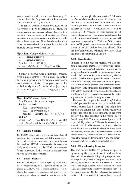
The general outline to obtain a composition of
two words is given in Algorithm 1. Here, we
first determine the sentence indices where the two
words w 1 and w 2 occur with relation r. Then,
we return the expectations around the two words
within these sentences. Note that the entire algorithm
can conveniently be written in the form of
database queries to our PropStore.
Algorithm 1 ComposePair(w 1 , r, w 2 )
M 1 ← queryMatrix(w 1 )
M 2 ← queryMatrix(w 2 )
SentIDs ← M 1 (r) ∩ M 2 (r)
return ((M 1 ∩ SentIDs) ∪ (M 2 ∩ SentIDs))
Similar to the two-word composition process,
given a parse subtree T of a phrase, we obtain
its matrix representation of empirical counts over
word-relation contexts. This procedure is described
in Algorithm 2. Let the E = {e 1 . . . e n }
be the set of edges in T , e i = (w i1 , r i , w i2 )∀i =
1 . . . n.
Algorithm 2 ComposePhrase(T )
SentIDs ← All Sentences in corpus
for i = 1 → n do
M i1 ← queryMatrix(w i1 )
M i2 ← queryMatrix(w i2 )
SentIDs ← SentIDs ∩(M 1 (r i ) ∩ M 2 (r i ))
end for
return ((M 11 ∩ SentIDs) ∪ (M 12 ∩ SentIDs)
· · · ∪ (M n1 ∩ SentIDs) ∪ (M n2 ∩ SentIDs))
3.4 Tackling Sparsity
The SDSM model reflects syntactic properties of
language through preferential filler constraints.
But by distributing counts over a set of relations
the resultant SDSM representation is comparatively
much sparser than the DSM representation
for the same word. In this section we present some
ways to address this problem.
3.4.1 Sparse Back-off
The first technique to tackle sparsity is to back
off to progressively more general levels of linguistic
granularity when sparse matrix representations
for words or compositional units are encountered
or when the word or unit is not in the
lexicon. For example, the composition “Balthazar
eats” cannot be directly computed if the named entity
“Balthazar” does not occur in the PropStore’s
knowledge base. In this case, a query for a supersense
substitute – “Noun.person eat” – can be
issued instead. When supersenses themselves fail
to provide numerically significant distributions for
words or word combinations, a second back-off
step involves querying for POS tags. With coarser
levels of linguistic representation, the expressive
power of the distributions becomes diluted. But
this is often necessary to handle rare words. Note
that this is an issue with DSMs too.
3.4.2 Densification
In addition to the back-off method, we also propose
a secondary method for “densifying” distributions.
A concept’s distribution is modified by
using words encountered in its syntactic neighborhood
to infer counts for other semantically similar
words. In other terms, given the matrix representation
of a concept, densification seeks to populate
its null columns (which each represent a worddimension
in the structured distributional context)
with values weighted by their scaled similarities to
words (or effectively word-dimensions) that actually
occur in the syntactic neighborhood.
For example, suppose the word “play” had an
“nsubj” preferential vector that contained the following
counts: [cat:4 ; Jane:2]. One might then
populate the column for “dog” in this vector with
a count proportional to its similarity to the word
cat (say 0.8), thus resulting in the vector [cat:4 ;
Jane:2 ; dog:3.2]. These counts could just as well
be probability values or PMI associations (suitably
normalized). In this manner, the k most similar
word-dimensions can be densified for each word
that actually occurs in a syntactic context. As with
sparse back-off, there is an inherent trade-off between
the degree of densification k and the expressive
power of the resulting representation.
3.4.3 Dimensionality Reduction
The final method tackles the problem of sparsity
by reducing the representation to a dense lowdimensional
word embedding using singular value
decomposition (SVD). In a typical term-document
matrix, SVD finds a low-dimensional approximation
of the original matrix where columns become
latent concepts while similarity structure between
rows are preserved. The PropStore, as described in
Section 3.1, is an order-3 tensor with w 1 , w 2 and
23