Team 13955: Computing Along the Big Long River

Computing Along the Big Long River
Control #13955
February 13 th , 2012
Abstract
In this paper, we develop a model to address the question of how
to best schedule trips down the Big Long River. The goal is to optimally
plan boat trips of varying duration and propulsion such that the number
of trips possible over the six month season is maximized. We begin by
modeling the process by which groups travel from campsite to campsite.
Given the constraints outlined above, as well as a limited amount of
campsites, our algorithm outputs the optimal daily schedule for each
group on the river. By studying our algorithm’s long term behavior, we
can compute a maximum number of trips, which we define as the river’s
“carrying capacity.” We apply our algorithm to a case study of the Grand
Canyon, which has many attributes in common with the Big Long River.
Finally, we examine carrying capacity’s sensitivity to changes in the
distribution of propulsion, trip duration, and the number of campsites on
the river’s corridor.

Page 2 of 18 Control #13955
Contents
1 Introduction 3
1.1 Defining the Problem . . . . . . . . . . . . . . . . . . . . . . . . . . . . . . . . . 3
1.2 Model Overview . . . . . . . . . . . . . . . . . . . . . . . . . . . . . . . . . . . . 3
1.3 Constraints . . . . . . . . . . . . . . . . . . . . . . . . . . . . . . . . . . . . . . 4
1.4 Assumptions . . . . . . . . . . . . . . . . . . . . . . . . . . . . . . . . . . . . . 4
1.5 Variables . . . . . . . . . . . . . . . . . . . . . . . . . . . . . . . . . . . . . . . 5
2 Methods 6
2.1 The Furthest Empty Campsite. . . . . . . . . . . . . . . . . . . . . . . . . . . . . 6
2.2 Priority . . . . . . . . . . . . . . . . . . . . . . . . . . . . . . . . . . . . . . . . . 7
2.3 Priorities & Other Considerations. . . . . . . . . . . . . . . . . . . . . . . . . . . 8
3 Scheduling Simulation 10
4 Case Study 12
4.1 The Grand Canyon . . . . . . . . . . . . . . . . . . . . . . . . . . . . . . . . . . .12
4.2 Sensitivity Analysis of Carrying Capacity With Respect to R and D . . . . . . . . . 13
4.3 Sensitivity Analysis of Carrying Capacity With Respect to R and Y . . . . . . . . . 15
5 Discussion & Conclusion 15
6 Limitations and Error Analysis 16
6.1 Carrying Capacity Overestimation . . . . . . . . . . . . . . . . . . . . . . . . . . . 16
6.2 Environmental Concerns . . . . . . . . . . . . . . . . . . . . . . . . . . . . . . . 16
6.3 Neglect of River Speed . . . . . . . . . . . . . . . . . . . . . . . . . . . . . . . . . 16
7 References 17
List of Figures
Figure 2.1 Example – applying priority & the scheduling algorithm . . . . . . . . . . . . . 7
Figure 2.2 Example – applying priority & the scheduling algorithm . . . . . . . . . . . . . 7
Figure 2.3 Example – applying priority & the scheduling algorithm . . . . . . . . . . . . . 8
Figure 2.4 Visual depiction of scheduling algorithm . . . . . . . . . . . . . . . . . . . . . 9
Figure 3.1 Hypothetical simulation . . . . . . . . . . . . . . . . . . . . . . . . . . . . . . .10
Figure 3.2 Hypothetical simulation results (from Figure 3.1) . . . . . . . . . . . . . . . . . 11
Figure 3.3 Hypothetical simulation results (From Figure 3.1) . . . . . . . . . . . . . . . . . 11
Figure 4.1 Grand Canyon case study results from simulation. . . . . . . . . . . . . . . . . 12
Figure 4.2 Ratio R to number of campsites Y . . . . . . . . . . . . . . . . . . . . . . . . . 13
Figure 4.3 Contour representation of Figure 4.2 . . . . . . . . . . . . . . . . . . . . . . . . 14
Figure 4.4 Ratio R to variation of trip days D . . . . . . . . . . . . . . . . . . . . . . . . . 15

Page 3 of 18 Control #13955
1 Introduction
Scheduling trips is an important task for the tourism industry, but the matter of scheduling is
also one of the more challenging problems to tackle. Airline companies juggle countless planes,
destinations, passengers and times of day to try to best optimize their costs as well as how many people
they are able to transport. Computer systems manage limited resources, multiple jobs, ‘due dates’ and
prioritization of jobs in order to function as a powerful and useful tool. Similar to these examples, river
managers have to be able to schedule river trips based on some of these same constraints while striving
to maximize the number of trips possible over a given time period.
The contents of this paper address the Big Long River, and our devised method of addressing
the issue of scheduling an optimal amount of trips per season. At 225 miles in length from First Launch
to Final Exit, passengers take oar-powered rubber rafts and motorized boats downstream. Trips last
between 6 and 18 nights, with tourists spending nights at campsites along the river corridor. To ensure
that campers enjoy a wilderness experience, it is desired that at most one group occupy any given
campsite each night. This constraint limits the number of possible trips during the park’s six month
season.
After the analysis of our model, we compare our results to rivers that have similar attributes to
that of the Big Long River, allowing us to verify that the approach does in fact yield desirable results.
In addition to this report we have attached a memo for the managers of the river. In the memo we
address the topics in which they were seeking advice, which consists of ways in which to develop the
best schedule for the river, and ways to determine the carrying capacity of the river.
Models focused on producing solutions to scheduling problems are quite complex. They must
be customized to address a vast number of variables in order to produce results subject to many
constraints. We have developed a model which speaks specifically to the constraints outlined thus far
and introduce what we believe to be reasonable assumptions in order to address the specific problem at
hand. With that said, our model is easily adaptable to find optimal trip schedules for rivers of varying
length, numbers of campsites, trip durations, and boat propulsions.
1.1 Defining the Problem
●
●
●
How should trips of varying length and propulsion be scheduled to maximize the number trips
possible over a six month season?
How many new groups can start a river trip on any given day?
What is the carrying capacity of the river?
○ We define carrying capacity as the maximum number of groups which can be sent down
the river during its six month season.
1.2 Model Overview
We have designed a model which:
• Can be applied to real-world rivers with similar attributes (i.e. the Grand Canyon).
• Is flexible enough to simulate a wide range of feasible inputs.

Page 4 of 18 Control #13955
• Simulates river trip scheduling as a function of some distribution of trip lengths (either 6, 12, or
18 days), a varying distribution of propulsion, and a varying number of campsites.
Ultimately, the model predicts the number of successful trips in a six month time frame. As a
result of finding this number, we also answer questions about the carrying capacity of the river,
advantageous distributions of propulsion and trip lengths, how many groups can start a river trip each
day, and how to schedule trips in such a way that these results are possible.
1.3 Constraints
The problem specifies the following constraints:
• Trips begin at First Launch and end at Final Exit – exactly 225 miles downstream.
• There are only two types of boats: oar-powered rubber rafts and motorized boats.
• Oar-powered rubber rafts travel 4 mph on average.
• Motorized boats travel 8 mph on average.
• Group trips will range from 6 to 18 nights.
• Trips are only scheduled during a six month period of the year.
• Campsites are distributed uniformly throughout the river corridor.
• No two sets of campers can occupy the same site at the same time.
1.4 Assumptions
• We have the ability to determine the proportion of oar-powered river rafts to motorized boats
that go onto the river each day.
Moving a high volume of groups down the river in a satisfactory time becomes an issue
if too many oar-powered boats are launched with short trip lengths.
• The duration of trips is constrained to the following values: 12 or 18 days for groups travelling
by oar-powered river rafts, and 6 or 12 days for those travelling by motorized boat.
This is a simplification which allows our model to produce more meaningful results
while preserving the ability to compare the effect of varying inputs.
• There can only be one group per campsite per night.
Our algorithm only considers campsites which are empty as open campsites that groups
can move to, which is consistent with the desires of the river manager.
• Each day, groups may only move downstream or remain in their current campsite -- they may
not move back up stream.
This allows us to restrict the flow of groups on the river to a single direction which
greatly simplifies the ways in which we can move groups from campsite to campsite.
• Groups heading downstream can only travel the river between 8am and 6pm.
This amounts to a maximum of 9 hours of travel per day (one hour is subtracted for
breaks/lunch/etc.). This implies that oar-powered river raft groups can travel at most 36 miles

Page 5 of 18 Control #13955
per day, and motorized boats can travel at most 72 miles per day. This allows us to determine
the set of groups that can reasonably reach a given campsite.
• Groups will never travel further than the amount of miles that they can feasibly travel in a
single day.
As the previous assumption states, this is 36 miles per day for oar-powered river rafts
and 72 miles per day for motorized boats in our model.
• Variables which could influence maximum daily travel distance, such as weather and river
conditions, are ignored.
There is no way of accurately including this in the model with the amount of given
information about the Big Long River.
• Campsites are distributed uniformly so that the distance between campsites is 225/Y (the
length of the river divided by the number of camp sites between the start and end of the river).
This assumption allows us to easily represent the river as an array of campsites that are
equally spaced out in our computer simulation.
• A group must reach the end of the river on the final day of its trip:
o A group will not leave the river early even if they are able to.
o A group will not have a finish date that is past their desired trip length.
This is an assumption that was made to best fit what we believed was an important
standard for the river manager and the quality of the trips that they will be scheduling.
1.5 Variables
• g ! = group number i
• t ! = total trip length for group i, measured in nights where 6 ≤ t ≤ 18
• d ! = number of nights group i has spent on the river
• Y = number of campsites on the river
• c ! = location of campsite Y in miles downstream 0 < c ! < 225
• c ! = a campsite representing First Launch (used to construct a waitlist of groups)
• c !"#$% = a campsite representing Final Exit (which is always ‘open’)
• l ! = location of group i's current campsite in miles down the river, where 0 < l < 225
• a ! = average distance that group i should move each day to be on schedule (a ! = 225 t ! )
• m ! = maximum distance that group i can travel in a single day
● P ! = priority of group i (where P ! = d ! t ! l ! 225 > 0)
This is a measure of how far ahead or behind schedule a group is. We will define priority P as
follows:
○ P ! > 1 implies that group g ! is behind schedule
○ P ! < 1 implies that group g ! is ahead of schedule
○ P ! = 1 implies that group g ! is precisely on schedule
● G ! = set of groups that can reach campsite c
● R = the ratio of oar powered river rafts to motorized boats launched each day
● X = the current number of trips down Big Long River each year

Page 6 of 18 Control #13955
●
●
M = peak carrying capacity of the river (maximum number of groups which can be sent down
the river during its six month season)
D = distribution of trip durations of groups on the river
2 Methods
Below is a description of the scheduling algorithm and, ultimately, our model which we have
found to be representative of accurate results based on the various inputs and assumptions specified
above. We begin by defining the following terms and phrases in an effort to add clarity to how certain
variables are handled in our simulation, as well as to shed light on some of the details of the
implementation of our model:
Open Campsite:
A campsite is considered to be an open campsite if there is no group currently occupying that
space. This is equivalent to saying that for a given campsite c ! there exists no other group g ! such that
g ! is assigned to c ! .
Moving to an open campsite:
For a group g ! and a campsite c ! , moving to an open campsite is equivalent to assigning g ! to
a new campsite, c ! . Since a group is only able to move downstream, or remain at their current
campsite, if g ! was previously occupying c ! , then g ! can only be moved to a c ! where m ≥ n.
Waitlist:
The waitlist for a given day is composed of the groups which are not yet on the river, but will
start their trip on day where their ranking on the waitlist and their ability to reach a campsite, c,
includes them in the set G ! , and is deemed ‘the highest priority’ (Note: priority is a significant element
of our model. This will be explained in further detail a little later). Waitlisted groups are initialized with
a current campsite value of c ! (the zero th campsite), and are assumed to have priority P = 1 until
they are moved from the waitlist onto the river.
Off the River:
Our algorithm considers the first space off of the river to be the ‘final campsite’, c !"#$% . For our
model, we consider c !"#$% to always be an open campsite, so that an infinite number of g ! can be
assigned to c !"#$% . This is consistent with the understanding that any number of groups can move off of
the river in a single day, and allows us to handle such an event in our simulation.
2.1 The Furthest Empty Campsite
Our scheduling algorithm utilizes an array as a data structure to represent the river, where each
element of the array consists of a campsite. The algorithm begins each day by finding the open
campsite that is furthest down the river, call that campsite c, then generates a set G ! , which consists of
all groups g ! which could potentially reach campsite c. Thus,
G ! = g ! | g ! , g ! , … , g ! ∶ where m ! + l ! ≥ c

Page 7 of 18 Control #13955
A couple of points about G ! remain to be made:
(1) The requirement of m ! + l ! ≥ c specifies that group g ! must be located at l ! and that must be
within at least m ! miles of campsite c.
(2) G ! can consist of groups that are both on the river and on the waitlist.
(3) If G ! = ∅, then we move to the next furthest empty campsite (Note: the next furthest empty
campsite that we look for is located up stream, closer to the start of the river – the algorithm
always runs from the end of the river, up towards the start of the river).
(4) If G ! ≠ ∅, then the algorithm will attempt to move the group with the highest priority to
campsite c. (For more instruction on this, see section 2.2: Priority).
The scheduling algorithm continues in this fashion until the furthest empty campsite is the zero th
campsite, c ! . At this point, every group that was able to move on the river that day has been moved to a
campsite, and we start the algorithm again from the beginning to simulate the next day.
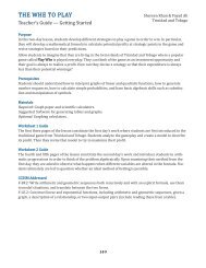
2.2 Priority
As noted in the last section, once the set G has been formed for a specific c, our algorithm must
decide which gεG to move to c. For this reason, we have developed the notion of priority for a group.
Then we essentially look at the priority of each gεG, take the g ! with the highest priority, and
attempt to move that group into c.
Some examples of situations that arise, and how the notion of priority is used to resolve them, are
outlined in Figures 2.1 & 2.2.
Campsite #: 1 2 3 4 5 6
Group
Assigned:
Downstream→
Group A
P ! = 1.1
Group B
P ! = 1.5
(moves to
campsite 6)
Group C
P ! = .8
Open Open Furthest
Open
Campsite
Figure 2.1: By running the scheduling algorithm we have found that furthest open campsite is campsite
6. The algorithm has found that Groups A, B and C can feasibly reach campsite 6. The priority of each
group is calculated, and Group B has the highest priority; thus, we move Group B to campsite 6.
Campsite #: 1 2 3 4 5 6
Group Group A
Assigned: P ! = 1.1
(moves to
campsite 5)
Downstream→
Open
Group C
P ! = .8
Open
Furthest
Open
Campsite
Group B

Page 8 of 18 Control #13955
Figure 2.2: As the scheduling algorithm progresses past campsite 6, we find that the next furthest open
campsite is campsite 5. The algorithm has calculated that Groups A and C can feasibly reach campsite
5. Since P ! >P ! , group A is moved to campsite 5.
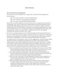
2.3 Priorities & Other Considerations
By knowing the group priority, our algorithm will always try to move the group that is the most
behind schedule. This is to ensure that each group is camping on the river for a number of days equal to
its predetermined trip length. However, in some instances it may not be ideal to move the g ! ∈ G which
has the highest priority to the campsite c which is the furthest empty campsite. Such is the case if g !
∈ G is the element with the highest priority, yet it is still ahead of schedule (P ! < 1).
To address the various caveats of handling group priorities in our scheduling algorithm, we
provide the following rules:
(1) If g ! is behind schedule, i.e. P ! > 1, then move g ! to c.
(2) If g ! is ahead of schedule, i.e. P ! < 1, then compute the following: d ! ∗ a ! . If the result is
greater than or equal to the location of campsite c (in miles), then move g ! to c. This
amounts to only moving g ! in such a way that it is no longer ahead of schedule.
(3) Regardless of P ! , if the chosen c = c !"#$% , then it will not move g ! → c unless t ! = d ! . This
ensures that trips will not end before their designated end date.
Campsite #: 170 171
…
223 224 Off the River
Group
Assigned:
Group D:
P ! = 1.1
t ! = 12
d ! = 11
(doesn't
move off the
river)
Downstream→
Open Open Open Open Furthest Open
Campsite
Figure 2.3: The furthest open campsite is the campsite that is off of the river. The algorithm finds that
Group D could move there, but since Group D has t ! > d ! , group D remains on the river.

Page 9 of 18 Control #13955
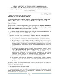
Figure 2.4: Visual depiction of scheduling algorithm.

Page 10 of 18 Control #13955
3 Scheduling Simulation
We will now use our model to briefly demonstrate how it could be used to schedule river trips.
In the following example, we assume there are 50 campsites along the 225 mile river, and introduce 4
groups to the river each day. We project the trip schedules of four specific groups, which we introduce
to the river on day 25. We choose a midseason date to demonstrate our models stability over time:
g ! : Motorized boat, t ! = 6
g ! : Oar-powered river raft, t ! = 18
g ! : Motorized boat, t ! = 12
g ! : Oar-powered river raft, t ! = 12
Campsite numbers and priority values for each group
Number of nights spent on river
g ! P ! g ! P ! g ! P ! g ! P !
1 5 1.43 2 1.32 3 1.28 1 3.85
2 20 0.71 6 0.87 19 0.4 8 0.96
3 20 1.07 6 1.32 19 0.61 8 1.44
4 36 0.79 13 0.81 19 0.81 15 1.02
5 36 0.99 13 1.01 19 1.01 15 1.28
6 49 0.87 13 1.21 35 0.66 23 1
7 OFF 1 13 1.42 35 0.77 25 1.08
8 13 1.66 35 0.88 32 0.96
9 15 1.58 35 0.99 32 1.08
11 23 1.14 35 1.1 39 0.99
12 30 0.96 49 0.86 39 1.08
13 30 1.05 49 0.94 46 1
14 30 1.14 OFF 1 OFF 1
15 36 1.02
16 36 1.1
17 44 0.96
18 44 1.02
19 44 1.01
20 OFF 1
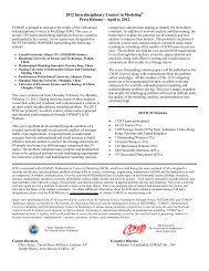
Figure 3.1: Shows each group’s campsite number and priority value for each night spent on the river.
I.e. the column labeled g ! gives campsite numbers for each of the nights of g ! ’s trip.
We find that each g ! is off the river after spending exactly t ! nights camping, and that P ! → 1 as
d ! → t ! . These findings are consistent with the intention of our method as outlined in section 2:
Methods. We see in this simulation that our algorithm produces desirable results. Figures 3.1 and 3.2,
display our results graphically.

Page 11 of 18 Control #13955
Campsite
Number
50
45
40
35
30
25
20
15
10
5
0
Group loca4ons (Figure 3.1)
Group 1
Group 2
Group 3
Group 4
0 1 2 3 4 5 6 7 8 9 10 11 12 13 14 15 16 17 18 19 Night
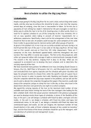
Figure 3.2: Movement of groups down the river based on Figure 3.1. Groups reach the end of
the river on different nights due to varying trip duration parameters.
Priority
4.5
4
3.5
3
2.5
2
1.5
1
0.5
0
Priority (Figure 3.1)
0 1 2 3 4 5 6 7 8 9 10 11 12 13 14 15 16 17 18 19
Night
P1
P2
P3
P4
Figure 3.3: Priority values of groups over the course of each trip. Values converge to P = 1
due to the algorithm’s attempt to keep groups on schedule.

Page 12 of 18 Control #13955
4 Case Study
4.1 The Grand Canyon
The Grand Canyon is an ideal case study for our model. It shares many characteristics with the
Big Long River. The Canyon’s primary river rafting stretch is 226 miles, has 235 campsites and is open
approximately six months out of the year. It allows tourists to travel by motorized boat, or oar powered
river raft for a maximum of 12 or 18 days respectively [3].
Using the parameters of the Grand Canyon, we tested our model by running a number of
simulations. We altered the number of groups we were placing on the water each day, attempting to
find a maximum “carrying capacity” for the river. We define “carrying capacity” as the maximum
number of possible trips down the Canyon’s river over a six month season. This is subject to the
constraint that each trip must end according to a group’s trip duration.
During its summer season, the Grand Canyon typically places six new groups on the water each
day [3], so we use this value for our first simulation. In each of the follow simulations we used an equal
distribution of motorized boats to oar powered river rafts, along with an equal distribution of trip
lengths.
Our model predicts the number of groups that make it off the end of the river (completed trips),
how many of those trips arrive past their desired end date (late trips), and the number of groups which
did not make it off the waitlist (total left on waitlist). These values change as we vary the number of
new groups placed on the water each day (groups/day).
Simulation # Groups/day Completed
trips.
Late Trips Total left on
waitlist
1 6 996 0 0
2 8 1328 0 0
3 10 1660 0 0
4 12 1992 0 0
5 14 2324 0 0
6 16 2656 0 0
7 17 2834 0 0
8 18 2988 0 0
9 19 3154 5 0
10 20 3248 10 43
11 21 3306 14 109
Figure 4.1: We predict that a maximum of 18 groups can be sent down the river each day. Over the
course of the six month season, this amounts to nearly 3000 trips.
We conclude that the maximum carrying capacity of the Grand Canyon is around 3000, and is
achieved by sending 18 new groups down the river each day. Increasing groups/day above 18 is likely
to cause late trips and long waitlists.
Notice that some groups are still on the river when our simulation ends. In simulation # 1, we
send a total of 1080 groups down that river (6 groups/day×180 days), but only 996 groups make it off.
This is simply because groups which began towards the end of the six month period have not reached
the end of their trip, so the groups are still on the river. These groups have negligible impact on our
simulation and they are essentially ignored.

Page 13 of 18 Control #13955
4.2 Sensitivity Analysis of Carrying Capacity With Respect to R and Y
Based on the similarities, we can assume that the managers of the Big Long River are faced
with a similar task as the managers of the Grand Canyon. Therefore, by finding an optimal solution for
the Grand Canyon, as we did in Section 4.1, it is possible that we have also found an optimal solution
for the Big Long River. However, this optimal solution is based on two key assumptions: that each day
we are putting approximately the same number of oar powered river rafts and motorized boats on the
river, and that the river has about one campsite per mile. We made these assumptions because they
were true for the Grand Canyon, but it is unknown to us whether or not they will be true for the Big
Long River.
To deal with these unknowns, we create the following table, Figure 4.2. The values in Figure
4.2 were generated by fixing Y (the number of campsites on the river), and R (the ratio of oar powered
river rafts to motorized boats launched each day), and then increasing the number of people added to
the river each day in our computerized algorithm until the river reaches its peak carrying capacity,
which is found the same way as in the Grand Canyon case study.
Ratio, R
(oar : motor)
Number of campsites on river, Y
100.00 150.00 200.00 250.00 300.00
1:4 1360.00 1688.00 2362.00 3036.00 3724.00
1:2 1181.00 1676.00 2514.00 3178.00 3854.00
1:1 1169.00 1837.00 2505.00 3173.00 3984.00
2:1 1157.00 1658.00 2320.00 2988.00 3604.00
4:1 990.00 1652.00 2308.00 2803.00 3402.00
Figure 4.2: Peak carrying capacity with respect to the number of campsites on the river and the ratio of
oar powered river rafts to motorized boats launched each day.
Since the peak carrying capacities in Figure 4.2 depend on two variables, we can visualize these
values as being data points in a 3-dimensional space. Consequently, we can find a best-fit surface that
passes through, or nearly through, this set of data points. This best fit surface will allow us to estimate
values of M, the peak carrying capacity of the river, for data points that are not represented in Figure
4.2. Essentially, it will give us M as a function of Y and R, and will show how sensitive the values of
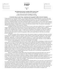
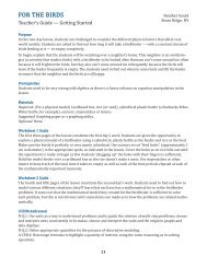
M are to changes in Y and/or R. Figure 4.3 is a contour diagram of this surface.

Page 14 of 18 Control #13955
Figure 4.3: Contour diagram of the best fit surface for data points in Figure 4.2, where contour lines
represent peak carrying capacity of the river (M). Notice that the surface has a ridge running along the
vertical line R=1:1.
Figure 4.3 is useful for visualizing how the river’s carrying capacity changes depending on the
two variables Y and R. The ridge along the vertical line R=1:1 predicts that for any given value of Y
between 100 and 300, the river will have an optimal value of M when R=1:1.
Unfortunately, the formula for this best fit surface is rather complex, and it doesn’t do an
accurate job of extrapolating beyond the set of data in Figure 4.2, so it is not a particularly useful tool
for predicting values of the river’s peak carrying capacity. As an alternative, if one wishes to predict
specific values of the river’s peak carrying capacity, the best method we have found is to use our
scheduling algorithm, which is more accurate than the best fit surface presented above and easier to
plug in values to.

Page 15 of 18 Control #13955
4.3 Sensitivity Analysis of Carrying Capacity With Respect to R and D
At this point, we have treated M as a function of R and Y, but it is still unknown to us how M is
affected by the mix of trip durations of groups on the river (D). For example, if we only scheduled trips
of 6 or 12 days, how would this affect M? The river managers want to know what mix of trips of
varying duration and propulsion will utilize the campsites in the best way possible. We can use our
scheduling algorithm to attempt to answer this question. We fix the number of campsites on the river at
200, and record what the peak carrying capacity of the river is for given values of R and D. The results
of this simulation are displayed in Figure 4.4.
Ratio
(oar : motor)
Distribution of trip lengths, D
12 12-18 6-12 6-18
1:4 2004 1998 2541 2362
1:2 2171 1992 2535 2514
1:1 2171 1986 2362 2505
2:1 1837 2147 2847 2320
4:1 2505 2141 2851 2308
Figure 4.4: Peak carrying capacity of river, M, with respect to D and R.
Figure 4.4 is intended to address the question of what mix of trip durations and propulsions will
yield a maximum carrying capacity for the river. The Big Long River managers could look to this table
to see approximately what value of M their current values of D and R will give, and also be able to see
how they could change their current values to increase the Big Long River’s peak carrying capacity.
For example:
• If the river managers are currently scheduling trips such that D ≈ 6 – 18, there value of M can
be increased either by increasing R to be closer to 1:1 or by decreasing D to be closer to 6-12.
• If the river managers currently have a D ≈ 12-18 then they should decrease their D to be closer
to 6-12.
• If the river managers currently have a D ≈ 6 – 12 then then can achieve a greater value of M by
increasing R to be closer to 4:1.
5 Conclusion
The river managers have asked how many more trips can be added to the Big Long River’s
season. Without knowing the specifics of how the river is currently being managed, we cannot give an
exact answer. However, by applying our model to a study of the Grand Canyon, we found results which
could be extrapolated to the context of the Big Long River. Specifically, we can say that the Big Long
River could add approximately 3000-X groups to the rafting season, where X is the current number of
trips, and 3000 is the carrying capacity of the Grand Canyon predicted by our scheduling algorithm.
Additionally, we’ve modeled how certain variables are related to each other. Namely, the relationship
between M, D, R and Y. River managers could refer to Figures 4.2 - 4.4 to see how they could update
their current values of D, R, and Y to achieve a greater carrying capacity for the Big Long River.

Page 16 of 18 Control #13955
We’ve also addressed the issue of scheduling campsite placement for groups moving down the
Big Long River through an algorithm which uses priority values to move groups downstream in an
orderly manner. Both our algorithm and its results should prove useful to the river managers as they
look to allow more trips this season.
6 Limitations and Error Analysis
6.1 Carrying Capacity Overestimation
Our model has several limitations. It assumes that the capacity of the river is constrained only
by number of campsites, trip durations, and transportation methods. We maximize the river’s carrying
capacity, even if this means that nearly every campsite is occupied each night. This may not be ideal,
potentially leading to congestion or environmental degradation of the river. Because of this, our model
may overestimate the maximum number of trips possible over long periods of time.
6.2 Environmental Concerns
Our case study of the Grand Canyon is evidence that our model omits variables. We are
confident that the Grand Canyon could provide enough campsites for 3000 trips over a six month
period, as predicted by our algorithm. However, since the actual figure is around 1000 trips [3], the
error is likely due to factors outside of campsite capacity, perhaps environmental concerns. If river
managers determined that 3000 trips per season would cause environmental harm to the Canyon, they
would scale back. This does not indicate a flaw in our modeling, but simply a limitation. Our results
represent a maximum number of trips, based on available campsites, and should be considered along
with other factors.
6.3 Neglect of River Speed
Another variable our model ignores is the speed of the river. River velocities increase with the
depth and slope of the river channel, making our assumption of constant maximum daily travel distance
impossible[6]. When a river experiences “high flow,” river speeds can double, and entire campsites can
end up under water[2]. Again, the results of our model don’t reflect these issues.

Page 17 of 18 Control #13955
7 References
[1] "Fitting a Surface to Scattered X-Y-Z Data Points." University of Colorado at Boulder. Web. 12
Feb. 2012. .
[2] "High Flow River Permit Information." Grand Canyon National Park. Web. 12 Feb. 2012.
.
[3] Jalbert, Linda, Lenore Grover-Bullington, and Lori Crystal. Colorado River Management Plan.
Publication. 2006. Web. 11 Feb. 2012.
.
[4] National Park Service. Grand Canyon National Park. 2011 Campsite List. Web. 11 Feb. 2012.
.
[5] National Park Service. Grand Canyon River Office. Grand Canyon River Statistics Calendar Year
2010. By Steve Sullivan. 27 May 2011. Web. 11 Feb. 2012.
.
[6] "River." Wikipedia. Web. 13 Feb. 2012. .

Page 18 of 18 Control #13955
Memo
To the river managers of the Big Long River,
In response to your questions regarding trip scheduling and river capacity, I am writing to
inform you of our findings.
Our primary accomplishment is the development of a scheduling algorithm. If implemented at
Big Long River, it could advise park rangers on how to optimally schedule trips of varying length and
propulsion. The optimal schedule will maximize the number of trips possible over the six month
season.
Our algorithm is flexible, taking a variety of different inputs. These include the number and
availability of campsites, and parameters associated with each tour group. Given the necessary inputs,
we can output a daily schedule. In essence, it does this using the state of the river from the previous
day. Schedules consist of campsite assignments for each group on the river, as well those waiting to
begin their trip. Given knowledge of future waitlists, our algorithm can output schedules months in
advance, allowing management to schedule the precise campsite location of any group on any future
date.
Sparing you the mathematical details, allow me to simply say that our algorithm uses a priority
system. It prioritizes groups who are behind schedule by allowing them to move to further campsites,
and holds back groups who are ahead of schedule. In this way it ensures that all trips will be completed
in precisely the length of time the passenger had planned for.
But scheduling is only part of what our algorithm can do. It can also compute a maximum
number of possible trips over the six month season. We call this the “carrying capacity” of the river. If
we find we are below our carrying capacity, our algorithm can tell us how many more groups we could
be adding to the water each day. Conversely, if we are experiencing river congestion, we can determine
how many fewer groups we should be adding each day to get things running smoothly again.
An interesting finding of our algorithm was how the ratio of motorized boats to oar powered
river rafts will affect the number of trips we can send downstream. When dealing with an even
distribution of trip durations (from 6 to 18 days), we recommend a 1:1 ratio to maximize the river’s
carrying capacity. If this distribution is skewed towards shorter trip durations then our model predicts
that increasing towards a 4:1 ratio will cause the carrying capacity to increase. If the distribution is
skewed the opposite way, towards longer trip durations, then the carrying capacity of the river will
always be less than in the previous two cases, so this is not recommended.
Our algorithm has been thoroughly tested and we believe it is a powerful tool for determining
your river’s carrying capacity, optimizing daily schedules, and ensuring that people will be able to
complete their trip as planned while enjoying a true wilderness experience. J
Yours Truly,
Control #13955