Fundamentals of Lightweight Design Formulary - lehrstuhl und ...

Fundamentals of Lightweight
Design
Formulary
Institut für Leichtbau, RWTH Aachen

Contents
1 General Formulas 1
2 Trusses 3
3 Bending of Beams 4
4 Transfer and Stiffness Matrices 10
5 Beams Subjected to Transverse Shear Forces 12
6 Torsion of Beams 18
7 Stiffened Shear Webs 23

1 General Formulas
1 General Formulas
– numerical integration rule:
f
F i+1 =
F i + 1 2 (f(z) i + f(z) i+1 ) · ∆z
i i+1 z
z
– isotropic materials:
– Hooke’s law (one-dimensional):
G =
E
2(1+ν)
σ x = ε x E
– strain-deformation relation for a bar:
ε x = du
dx
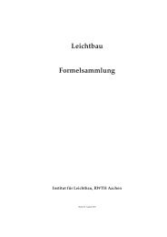
– standard box for the determination of cutting forces:
– differential equations for the equilibrium of beams:
dQ z
dx = −p(x)
dM y
dx
= Q z
1

1 General Formulas
– definition of Young’s moduli in the plastic range:
· tangent modulus:
E T = dσ
dε
· secant modulus
E S = σ ε
– stress-strain relation according to Ramberg-Osgood:
· stress-strain relation:
ε = σ 0,7
E
[ σ
+ 3 ( ) σ n ]
σ 0,7 7 σ 0,7
; n =1+
ln(
17
7 )
ln( σ 0,7
σ 0,85
)
· tangent modulus:
E T =
E
1+ 3 7 n (
σ
σ 0,7
) n−1
· secant modulus:
E S =
1+ 3 7
E
( ) n−1 σ
σ 0,7
· σ 0,7 and σ 0,85 are defined as shown in the following figure:
2

2 Trusses
2 Trusses
– degree of redundancy:
U = n + A − 2k
U = n + A − 3k r − 2k e
A: number of reaction forces
n: numberofbars
k: numberofnodes
k r : number of three-dimensional nodes
k e : number of two-dimensional nodes
(two-dimensional)
(three-dimensional)
– equilibrium of nodes (two-dimensional):
∑
X = P cos(ϕ)+
∑
Ni cos(γ i )=0
∑
Y = P sin(ϕ)+
∑
Ni sin(γ i )=0
– three-dimensional decomposition of a force / similarity of the bar force components
(F ix , F iy , F iz ) to the bar lengths (l ix , l iy , l iz ):
√
l i = lix 2 + l2 iy + l2 iz
cos α = F ix
F i
= l ix
l i
; cosβ = F iy
F i
= l iy
; cosγ = F iz
= l iz
l i F i l i
3

3 Bending of Beams
3 Bending of Beams
– statical moments of an area:
∫
S y =
– moments of inertia of an area:
∫
I y =
– product of inertia of an area:
A
A
∫
zdA S z =
∫
z 2 dA I z =
∫
I yz =
A
yz dA
A
A
ydA
y 2 dA
– stress distribution for an arbitrary coordinate system in the center of gravity:
σ x (z,y) = N A + M yI z + M z I yz
I y I z − I 2 yz
z − M zI y + M y I yz
I y I z − Iyz
2 y
– stress distribution for a system of principal axes in the center of gravity:
– section moduli:
– polar moment of inertia:
σ x (z,y) = N A + M y
I y
z − M z
I z
y
W y =
I y
|z max |
∫
I p = I y + I z =
– radii of gyration:
i 2 y = I y
A
– location of the centroid of an area:
∫
A
η s =
ηdA
A
W z =
A
r 2 dA
i 2 z = I z
A
ζ s =
I z
|y max |
∫
A ζdA
A
– coordinate transformation for a rotation of the coordinate system about ϕ:
z = −y ′ sin ϕ + z ′ cos ϕ
y = y ′ cos ϕ + z ′ sin ϕ
4

3 Bending of Beams
– theorem of Steiner:
I η = I y ′ + ζ 2 s A I ζ = I z ′ + η 2 sA I ηζ = I y ′ z ′ + η sζ s A
– change of the moments of inertia and of the product of inertia due to a rotation of the
coordinate system:
I y (ϕ) = 1 ( 1
Iy ′ + I z ′)
+
2
2
I z (ϕ) = 1 ( 1
Iy ′ + I z ′)
−
2
2
I yz (ϕ) = 1 (
Iy ′ − I z ′
2
– location of the principal axes:
– differential equation of the deflection line:
( )
Iy ′ − I z ′ cos 2ϕ − Iy ′ z ′ sin 2ϕ
( )
Iy ′ − I z ′ cos 2ϕ + Iy ′ z ′ sin 2ϕ
)
sin 2ϕ + Iy ′ z ′ cos 2ϕ
tan 2α = − 2I y ′ z ′
I y ′ − I z ′
w ′′′′ I y E = p(x) ⇒ w ′′′ = − Q z
I y E
⇒
w ′′ = − M y
I y E
Plastic Bending:
– relation between longitudinal force and longitudinal stress:
∫
N = σ(z)dA
– relation between bending moment and longitudinal stress:
∫
M = σ(z) · zdA
A
A
– definitions:
– interaction curves:
ν =
N
µ = M
A · σ B W · σ B
· elastic material behaviour:
ν + µ =1
· ideal plastic material behaviour (valid only for a rectangular cross section):
µ =6 ( κ − κ 2) }
ν =(2κ − 1)
⇒ µ =1.5 ( 1 − ν 2) 5

3 Bending of Beams
– It applies for ν =0:
· ideal plastic material behaviour:
· Cozzone’s approximation:
M plastic =
M plastic = K · M elastic
[
1+(K − 1) σ ]
o
M elastic
σ M
· Values of K for some typical cross sections are given on page 9.
6

3 Bending of Beams
moments of inertia for typical cross sections:
I y = ba3
12
I z = ab3
12
I y = ba3
36
I z = ab3
48
I y = I z = π 4
( R
4
a − R 4 i
)
I y = π 4
(
aa b 3 a − a ib 3 i
)
I z = π 4
(
a
3
a b a − a 3 i b i)
s
thin-walled circle:
y
R
I y = πR 3 s
z
I z = πR 3 s
a
thin-walled ellipse:
y
b
I y = π 4 sb2 (b +3a)
s
z
I z = π 4 sa2 (a +3b)
7

3 Bending of Beams
deflection lines for selected load cases:
w =
Fl
6EI y
x ( )
2 3 − x l
w = − M
2EI y
x 2
(
w =
pl2
24EI y
x 2 6 − 4 x + ( ) )
x 2
l l
w =
(
pl2
120EI y
x 2
10 − 10 x l +5( x
l
) 2
− ( ) )
x 3
l
(
x ≤ a : w = Flb
6EI y
x 1 − ( )
b 2 (
l − x
) ) 2
l
(
w = Fl2 a
6EI y
1 −
x
l
x ≥ a :
) ( 1 − ( a
l
) 2 ( ) )
− 1 −
x 2
l
w =
pl3
24EI y
x ( 1 − x l
) ( 1+ x − ( ) )
x 2
l l
w =
(
pl3
360EI y
x
7 − 10 ( x
l
) 2
+3 ( ) )
x 4
l
8

3 Bending of Beams
values of K (plastic bending) for typical cross sections:
sketch
K
thin web
K =1.0
[
K =1.5
]
h 3 t 2 +4ht 1·(b−t 2 )(h−t 1 )
h 3 t 2 +2t 1 (b−t 2 )(3h 2 −6ht 1 +4t 2 1 )
K =1.5
[ ]
h 3 t 2 +ht 2 1 (b−t 2)
h 3 t 2 +t 3 1 (b−t 2)
K =1.5
thin walled tubes
K =1.27
K =1.698 D(D3 −d 3 )
D 4 −d 4
K =1.698
K =2.0
9

4 Transfer and Stiffness Matrices
4 Transfer and Stiffness Matrices
Transfer Matrices {W } and State Vectors → u:
– bar with a constant distributed longitudinal load:
– shear-rigid beam:
→
u=
⎡
⎣
u
N
1
⎤
⎧
⎨
⎦ {W } =
⎩
l
1
AE
−p L l 2
2AE
0 1 −p L l
0 0 1
⎫
⎬
⎭
⎡
→ u= ⎢
⎣
w
w ′
M y
Q z
1
⎤
⎥
⎦
w = w B
(a) transfer matrix for a constant distributed transverse load:
⎧
⎪⎩
1 l
−l 2
2I yE
0 1
−l
I yE
−l 3
6I yE
−l 2
2I yE
⎪⎨
{W } =
0 0 1 l
p 0 l 4
24I yE
p 0 l 3
6I yE
−p 0 l 2
2
0 0 0 1 −p 0 l
0 0 0 0 1
⎫
⎪⎬
⎪⎭
(b) dot matrix {P } in order to consider the introduction of concentrated loads:
⎧
⎪⎨
{P } =
⎪⎩
1 0 0 0 0
0 1 0 0 0
0 0 1 0 M
0 0 0 1 −P
0 0 0 0 1
⎫
⎪⎬
⎪⎭
10

4 Transfer and Stiffness Matrices
– shear-flexible beam:
⎡
→ u= ⎢
⎣
w
w ′ B
M y
Q z
1
⎤
⎥
⎦
w = w B + w S
⎧
⎪⎩
1 l
−l 2
2I yE
0 1
−l
I yE
(
−l 3
6I yE +
⎪⎨
{W } =
0 0 1 l
−l 2
2I yE
l
A Qz G
)
(
p 0 l 4
I yE 24 − IyEl2
2A Qz G
p 0 l 3
6I yE
−p 0 l 2
2
0 0 0 1 −p 0 l
0 0 0 0 1
)
⎫
⎪⎬
⎪⎭
Stiffness Matrices:
– shear-rigid beam with a constant distributed transverse load:
⎡
⎢
⎣
⎤
Q 0
M 0
Q 1
M 1
⎥
⎦ = EIy
⎡
⎧⎪
12 −6l −12 −6l
⎨
⎫⎪
−6l 4l 2 6l 2l 2 ⎬ ⎢
l 3 ⎪ −12 6l 12 6l ⎣
⎩ ⎪ ⎭
−6l 2l 2 6l 4l 2
w 0
w ′ 0
w 1
w ′ 1
⎤
⎥
⎦ + p 0l
2
⎡
⎢
⎣
−1
l
6
−1
− l 6
⎤
⎥
⎦
11

5 Beams Subjected to Transverse Shear Forces
5 Beams Subjected to Transverse Shear Forces
Open Thin-Walled Sections:
– shear flow formula:
t = Q zS y
I y
– rules for a qualitative description of the shear flow distribution:
(1) The shear flow is directly proportional to the statical moment.
(2) At an open end the shear flow is equal to zero, as the statical moment is zero.
(3) The shear flow behaves linearly along the section center line for center lines that
are parallel to the line of zero stress.
(4) The shear flow has a parabolic shape for center lines that are perpendicular to
the line of zero stress, the slope
· decreases for integration towards the line of zero stress (lever arm gets smaller)
and
· increases for integration away from the line of zero stress (lever arm gets
larger).
(5) If the cross section is symmetric to the line of zero stress, the shear flow will be
symmetric as well.
(6) The direction of the shear flow corresponds to the direction of the loading: theory
of sources and drains.
(7) At branching points use the correct signs when superposing the statical moments.
12

5 Beams Subjected to Transverse Shear Forces
– shear center:
∫
s
resp.
t(s)ρ(s)ds = Q z · e y
e y = 1 I y
∫
s
S y ρds
Closed Thin-Walled Sections:
– Bredt’s first formula:
M t =2t 0 A
– procedure for the shear flow calculation of closed sections (only valid, if there are no
warping stresses, i.e. if the transverse force acts through the shear center or if the
cross section is a cross section of zero warping):
(1) The closed section is cut at any arbitrary point:
⇒ open section: t ′ = QzSy
I y
(2) The shear flow t 0 is determined by the equality of twisting moments.
∮
Q z a = t ′ ρds +2At 0 = Q z e 1 +2At 0
(3) The shear flows t ′ and t 0 are superposed.
– condition for the determination of the shear center:
ϑ ′ =0
⇒
∮ t
′
Q z
∮ Sy
+ t 0,SC
I
ds =0 ⇒ t 0,SC = −
y Gh
∮ ds
Gh
ds
Gh
13

5 Beams Subjected to Transverse Shear Forces
– Using this relation, the shear center can be determined by the following equation:
∮
∮
A Sy
Q z e = t ′ I
ρds +2t 0,SC A ⇒ e = e 1 − 2
y Gh ds
∮ ds
Gh
– condition for cross sections of zero warping:
∫ 2
1
ds
Gh = ∆A ∮
A
ds
Gh
Shear-Flexible Beams:
– The deformation w B of shear-rigid beams is superposed by the shear deformation w S :
w = w B + w S
– Hooke’s law (dependence of the shear deformation on the shear stress):
γ(z) = τ(z)
G
– average shear angle γ m and shear correction factor κ z :
w ′ τ
S = γ m = κ z
G = κ Q z
z
AG
– determination of κ z :
κ z = A Iy
2
∫
κ z = A I 2 y
s
∫
z
S 2 y
B dz
(solid cross sections)
Sy
2
h ds (thin-walled cross sections) 14

5 Beams Subjected to Transverse Shear Forces
– shear-bearing area:
A Qz = A κ z
– approximation for thin-walled cross sections:
κ z =
A
∑
Aweb
– differential equation of shear-flexible beams:
w ′′′′ = −
p′′
A Qz G + p
I y E
As boundary conditions the following expressions must be used:
w or Q z = w ′ sA Qz G
β = w ′ B = w′ − γ m or M y = −w ′′ B I yE
15

5 Beams Subjected to Transverse Shear Forces
shear center locations:
e =
3hb2
ah s +6bh
e = ab3 2
b 3 1 + b3 2
sin α − α cos α
e =2R
α − sin α cos α
e =2R
16

5 Beams Subjected to Transverse Shear Forces
shear correction factors (η = a b ): κ z = κ y =1.11
κ z = κ y =1.2
κ z = η +2
(6η + η 2 ) 2 (
24 + 36η +12η 2 + 6 5 η3 )
κ y =
3(η +2) 3
(2 + 5η +2η 2 ) 2 ( 1
5 + 7
10 η + 4 5 η2 + 1 4 η3 )
κ z = η +2
(6η + η 2 ) 2 (
6+36η +12η 2 + 6 5 η3 )
κ y = 3 (η +2)
5
κ z =
12(η +1) 3
η 2 (4 + 5η + η 2 ) 2 ( 1
4 + 8 5 η + 7
10 η2 + 1
10 η3 )
κ y = 6 (η +1)
5
y
κ z = κ y =2.0
z
17

6 Torsion of Beams
6 Torsion of Beams
Twisting Moment:
T = M t + Q y e z − Q z e y
Saint Vénant’s torsion:
– definitions:
· torsional moment of an area:
ϑ ′ =
T
GI T
(I T ≠ I p )
· torsional section modulus:
– closed thin-walled sections:
τ max =
T W T
· section modulus (h min : minimum wall thickness):
W T =2Ah min
· Bredt’s first formula:
· Bredt’s second formula:
M t =2t 0 A
GI T = 4A2 ∮ ds
Gh
18

6 Torsion of Beams
– prismatic bars of solid cross section:
· circular solid section:
· elliptical solid section:
I T = π 2 R4
W T = π 2 R3
I T = π a3 b 3
a 2 + b 2
W T = πab2
2
· rectangular solid section:
I T = η 1
B 3 H
3
W T = η 2
B 2 H
3
H/B η 1 η 2
1 0.4217 0.6245
1.25 0.5152 0.6636
1.5 0.5873 0.6929
2 0.6860 0.7376
3 0.7900 0.8016
4 0.8424 0.8450
5 0.8745 0.8740
6 0.8951 0.8950
8 0.9212 0.9212
10 0.9370 0.9370
∞ 1.0000 1.0000
19

6 Torsion of Beams
– approximations:
· narrow rectangular section:
I T = 1 3 B3 H
W T = B2 H
3
τ = τ max
2y
B
· thin-walled open sections:
1 ∑
I T = η 3 h 3 i l i
3
W T = I t
=
h max η ∑
3
h 3 i l i
3h max
i
i
section shape L U Z T I X
η 3 0.99 1.12 1.12 1.12 1.30 1.17
· thick-walled hollow sections:
ϑ ′ = ϑ ′ B = ϑ′ i
T = T B + ∑ i
T i
⎫
⎬
⎭ ⇒ I T = I TB + ∑ i
I Ti
τ max,i =
3T i
η 2i h 2 i l i
τ Bi =
T B
2HBh i
20

6 Torsion of Beams
Restrained-Warping Torsion
– twisting moments due to Saint Venant’s torsion M SV and due to bending torsion M B :
M SV = ϑ ′ GI T
M B = −ϑ ′′′ C T E
– differential equation of restrained-warping torsion:
d 3 ϑ dϑ
− α2
dξ3 dξ = −µ
with
ξ = x l
α 2 = GI T l 2
EC T
µ = Tl3
EC T
– solution for a clamped cantilever beam subjected to a constant twisting moment:
with
ϑ = A 1 + A 2 cosh αξ + A 3 sinh αξ + µ α 2 ξ
A 1 = −A 2 = − µ α 3 tanh α A 3 = − µ α 3 21

6 Torsion of Beams
warping resistance C T :
C T = a 2 I F 1I F 2
I F 1 + I F 2
C T = a 2 b 2 A F
( 1
6 −
)
A F
8A F +4A S
(
)
C T = a 2 b 2 1
A F
6 − A F
8A F + 4 3 A S
22

7 Stiffened Shear Webs
7 Stiffened Shear Webs
Open Stiffened Shear Webs
– shear flow:
t = Q a
– longitudinal force in the flanges:
N = M y
a
A
– shear center:
Q
a
e = 2A a
e
Closed Stiffened Shear Webs with 2 Flanges
– determination of the shear flow distribution
· method 1:
Q = Q 1 + Q 2 ; Qd = Q 1 e 1 − Q 2 e 2
23

7 Stiffened Shear Webs
· method 2:
Two-Dimensional Stiffened Shear Webs
– degree of redundancy:
U = S + B + A − 2k
S: numberofbars
B: numberofpanels
A: number of reaction forces
k: numberofnodes
– determination of the longitudinal bar forces:
N(x) =
– rectangular webs:
∫ x
0
tdx + N 0
t = t 1 = t 2 =
t 3 = t 4 =
const.
24

7 Stiffened Shear Webs
– parallelogram webs:
t = t 1 = t 2 =
t 3 = t 4 =
const.
n x =2t tan ϕ
– trapezoidal webs:
· definition of mean shear flow:
t =
∫ l
0 t(x)dx
l
· determination of the mean shear flows:
t 3
t 1
=
(
a1
a 3
) 2
t 1
t 2
= t 4
t 3
= a 3
a 1
t 2 = t 4
· The shear flows along the edges 1 and 3 are constant:
t 1 = t 1 = const.
t 3 = t 3 = const.
· shear flow distribution along the edges 2 and 4:
( ) 2 ( )
a3
d
2
t(x) =t 3 = t 3
a(x) d + x
t(x) =t m
a 1 a 3
a(x) 2 t m = √ t 2 t 4 = √ t 1 t 3
· longitudinal force in the bars 2 and 4:
N 2 (x) =N 20 + t 3
cos α
1+ x l
x
( ) N 4 (x) =N 40 − t 3
a1
a 3
− 1
cos β
1+ x l
x
( )
a1
a 3
− 1
25

7 Stiffened Shear Webs
– general quadrangular webs:
A = t 1 p A p B = t 2 p B p C =
t 3 p C p D = t 4 p D p A
t m = √ t 2 t 4 = √ t 1 t 3
· shear flow along the edge i:
t i (u i )=
t i0
[
1+(
pil
p i0
− 1
) ] 2 ui
l i
t i0 = A p 2 i0
· longitudinal force in the bar i:
N i (u i )=N i0 +
t i0 u i
1+(
pil
p i0
− 1
)
ui
l i
Three-Dimensional Stiffened Shear Webs
– degree of redundancy:
U = S + B + A − 3k r − 2k e
S: numberofbars
B: numberofpanels
A: number of reaction forces
k r : number of three-dimensional nodes
k e : number of two-dimensional nodes
26

7 Stiffened Shear Webs
shear center locations for some web shapes:
straight
web
arbitrary
shape
parabula semicircle large arc
e =0 e =2 A H
e = 4a 3
e = π 2 R
e = 2A
H t
Q = tH Q = tH Q = tH Q = tH Q = tH t
M αt =0
M αt = M αt = M αt =
2At
4
3 Hat R 2 πt
M αt =2At
load bearing capabilities of stiffened shear webs:
longitudinal force
in the centroid of
the flanges
transverse parallel to
force in 1-1
X
X
X X X X X
X
X X
X
the shear arbitrary
center direction
X X X X
perpendicular
to 1-1
bending
X X X
moment arbitrary
direction
X X X X
twisting moment X X X X X
27