Entropy Inference and the James-Stein Estimator, with Application to ...
Entropy Inference and the James-Stein Estimator, with Application to ...
Entropy Inference and the James-Stein Estimator, with Application to ...
Create successful ePaper yourself
Turn your PDF publications into a flip-book with our unique Google optimized e-Paper software.
HAUSSER AND STRIMMER<br />
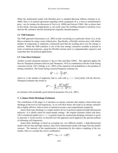
While <strong>the</strong> multinomial model <strong>with</strong> Dirichlet prior is st<strong>and</strong>ard Bayesian folklore (Gelman et al.,<br />
2004), <strong>the</strong>re is no general agreement regarding which assignment of a k is best as noninformative<br />
prior—see for instance <strong>the</strong> discussion in Tuyl et al. (2008) <strong>and</strong> Geisser (1984). But, as shown later<br />
in this article, choosing inappropriate a k can easily cause <strong>the</strong> resulting estima<strong>to</strong>r <strong>to</strong> perform worse<br />
than <strong>the</strong> ML estima<strong>to</strong>r, <strong>the</strong>reby defeating <strong>the</strong> originally intended purpose.<br />
2.4 NSB <strong>Estima<strong>to</strong>r</strong><br />
The NSB approach (Nemenman et al., 2002) avoids overrelying on a particular choice of a k in <strong>the</strong><br />
Bayes estima<strong>to</strong>r by using a more refined prior. Specifically, a Dirichlet mixture prior <strong>with</strong> infinite<br />
number of components is employed, constructed such that <strong>the</strong> resulting prior over <strong>the</strong> entropy is<br />
uniform. While <strong>the</strong> NSB estima<strong>to</strong>r is one of <strong>the</strong> best entropy estima<strong>to</strong>rs available at present in<br />
terms of statistical properties, using <strong>the</strong> Dirichlet mixture prior is computationally expensive <strong>and</strong><br />
somewhat slow for practical applications.<br />
2.5 Chao-Shen <strong>Estima<strong>to</strong>r</strong><br />
Ano<strong>the</strong>r recently proposed estima<strong>to</strong>r is due <strong>to</strong> Chao <strong>and</strong> Shen (2003). This approach applies <strong>the</strong><br />
Horvitz-Thompson estima<strong>to</strong>r (Horvitz <strong>and</strong> Thompson, 1952) in combination <strong>with</strong> <strong>the</strong> Good-Turing<br />
correction (Good, 1953; Orlitsky et al., 2003) of <strong>the</strong> empirical cell probabilities <strong>to</strong> <strong>the</strong> problem of<br />
entropy estimation. The Good-Turing-corrected frequency estimates are<br />
ˆθ GT<br />
k = (1 − m 1 ML<br />
)ˆθ k ,<br />
n<br />
where m 1 is <strong>the</strong> number of single<strong>to</strong>ns, that is, cells <strong>with</strong> y k = 1. Used jointly <strong>with</strong> <strong>the</strong> Horvitz-<br />
Thompson estima<strong>to</strong>r this results in<br />
Ĥ CS = −<br />
p<br />
∑<br />
k=1<br />
ˆθ GT<br />
k<br />
log ˆθ GT<br />
k<br />
(1 −(1 − ˆθ GT<br />
k<br />
) n ) ,<br />
an estima<strong>to</strong>r <strong>with</strong> remarkably good statistical properties (Vu et al., 2007).<br />
3. A <strong>James</strong>-<strong>Stein</strong> Shrinkage <strong>Estima<strong>to</strong>r</strong><br />
The contribution of this paper is <strong>to</strong> introduce an entropy estima<strong>to</strong>r that employs <strong>James</strong>-<strong>Stein</strong>-type<br />
shrinkage at <strong>the</strong> level of cell frequencies. As we will show below, this leads <strong>to</strong> an entropy estima<strong>to</strong>r<br />
that is highly effective, both in terms of statistical accuracy <strong>and</strong> computational complexity.<br />
<strong>James</strong>-<strong>Stein</strong>-type shrinkage is a simple analytic device <strong>to</strong> perform regularized high-dimensional<br />
inference. It is ideally suited for small-sample settings - <strong>the</strong> original estima<strong>to</strong>r (<strong>James</strong> <strong>and</strong> <strong>Stein</strong>,<br />
1961) considered sample size n = 1. A general recipe for constructing shrinkage estima<strong>to</strong>rs is given<br />
in Appendix A. In this section, we describe how this approach can be applied <strong>to</strong> <strong>the</strong> specific problem<br />
of estimating cell frequencies.<br />
<strong>James</strong>-<strong>Stein</strong> shrinkage is based on averaging two very different models: a high-dimensional<br />
model <strong>with</strong> low bias <strong>and</strong> high variance, <strong>and</strong> a lower dimensional model <strong>with</strong> larger bias but smaller<br />
variance. The intensity of <strong>the</strong> regularization is determined by <strong>the</strong> relative weighting of <strong>the</strong> two<br />
models. Here we consider <strong>the</strong> convex combination<br />
ˆθ Shrink<br />
k<br />
= λt k +(1 − λ)ˆθ ML<br />
k , (4)<br />
1472


