Elastic Registration of 3D Deformable Objects
Elastic Registration of 3D Deformable Objects
Elastic Registration of 3D Deformable Objects

Create successful ePaper yourself
Turn your PDF publications into a flip-book with our unique Google optimized e-Paper software.
<strong>Elastic</strong> <strong>Registration</strong> <strong>of</strong> <strong>3D</strong> <strong>Deformable</strong> <strong>Objects</strong><br />
Zsolt Sánta and Zoltan Kato<br />
Image Processing and Computer Graphics Dept., University <strong>of</strong> Szeged<br />
H-6701 Szeged, PO. Box 652., Hungary, Fax: +36 62 546-397<br />
Email: {santazs, kato}@inf.u-szeged.hu<br />
Abstract—A novel correspondence-less approach is proposed<br />
to find a non-linear aligning transformation between a pair<br />
<strong>of</strong> deformable <strong>3D</strong> objects. Herein, we consider a polynomial<br />
deformation model, but our framework can be easily adapted<br />
to other common deformations. The basic idea <strong>of</strong> the proposed<br />
method is to set up a system <strong>of</strong> nonlinear equations whose solution<br />
directly provides the parameters <strong>of</strong> the aligning transformation.<br />
Each equation is generated by integrating a nonlinear function<br />
over the object’s domains. Thus the number <strong>of</strong> equations is determined<br />
by the number <strong>of</strong> adopted nonlinear functions yielding a<br />
flexible mechanism to generate sufficiently many equations. While<br />
classical approaches would establish correspondences between<br />
the shapes, our method works without landmarks. The efficiency<br />
<strong>of</strong> the proposed approach has been demonstrated on a large<br />
synthetic dataset as well as in the context <strong>of</strong> medical image<br />
registration.<br />
I. INTRODUCTION<br />
<strong>Registration</strong> <strong>of</strong> deformable objects [1], [2] has many application<br />
areas such as <strong>3D</strong> laser scan registration [3] or<br />
volumetric medical image alignment [4]. When registering<br />
a pair <strong>of</strong> objects, first we have to characterize the possible<br />
deformations. From this point <strong>of</strong> view, registration techniques<br />
can be classified into two main categories: physical modelbased<br />
and parametric or functional representation [5]. Herein,<br />
we deal with the latter representation, which typically originate<br />
from interpolation and approximation theory. A broad<br />
class <strong>of</strong> such deformations are polynomial. Unlike splinebased<br />
transformations e.g. thin plate splines [6], [7], which<br />
are typically based on interpolation, polynomial models are<br />
approximating the underlying deformation. Furthermore, the<br />
control points <strong>of</strong> interpolating thin plate spline models are<br />
placed at extracted point matches and they usually include<br />
various regularizations, such as the bending energy [6]. On<br />
the other hand, polynomial deformations are governed by<br />
fewer parameters and are acting globally on the shapes, hence<br />
regularization is not needed. Moreover, many non-polynomial<br />
transformation can be approximated by a polynomial one e.g.<br />
via a Taylor expansion [8].<br />
From an algorithmic viewpoint, registration methods can be<br />
divided into two main categories: landmark-based and areabased<br />
(or feature-less) approaches. Landmark-based methods<br />
are challenged by the correspondence problem, which<br />
is particularly difficult to solve in the case <strong>of</strong> non-linear<br />
deformations. Area-based approaches are typically relying on<br />
the availability <strong>of</strong> rich radiometric information which is used to<br />
construct a similarity measure based on some kind <strong>of</strong> intensity<br />
correlations. The aligning transformation is then found by<br />
maximizing similarity between the objects, which usually<br />
yields a complex non-linear optimization procedure. In many<br />
cases, reliable radiometric information may not be available<br />
(e.g. range data or multimodal medical images), therefore<br />
purely shape-based methods are particularly interesting [1],<br />
[2], [3], [4], [9].<br />
Most <strong>of</strong> these approaches are focusing on point set registration.<br />
In [9], a probabilistic model is proposed where a Gaussian<br />
mixture with centroids corresponding to the first set is fit to<br />
the second point set by maximizing the likelihood. In [1], both<br />
point sets are represented as a Gaussian mixture model and<br />
then the L2 distance <strong>of</strong> the two mixtures is minimized. While<br />
point-based registration has the advantage <strong>of</strong> tolerating rather<br />
high occlusions, they are typically inefficient for large point<br />
sets. In many applications, however, the goal is the accurate<br />
alignment <strong>of</strong> whole volumetric objects <strong>of</strong> several megavoxels.<br />
Therefore object level registration methods are needed e.g. in<br />
medical imaging.<br />
While elastic registration <strong>of</strong> planar shapes has been addressed<br />
by many researchers [10], [8], the extension <strong>of</strong> 2D<br />
methods for <strong>3D</strong> object registration is far from trivial. Herein,<br />
we propose a correspondence-less approach for aligning <strong>3D</strong><br />
deformable objects subject to a polynomial deformation. The<br />
basic idea is to construct a system <strong>of</strong> nonlinear equations by<br />
integrating a set <strong>of</strong> nonlinear functions over the object volumes<br />
and then solve it by classical Levenberg-Marquardt algorithm.<br />
We have conducted a series <strong>of</strong> quantitative tests on a synthetic<br />
dataset to demonstrate the performance and robustness <strong>of</strong> the<br />
proposed approach. The method has been successfully applied<br />
to the alignment <strong>of</strong> segmented lung CT images.<br />
II. POLYNOMIAL REGISTRATION FRAMEWORK<br />
A broadly used class <strong>of</strong> deformations is the polynomial<br />
family. In the three dimensional case, the deformation field<br />
π : R 3 → R 3 , π(x) = [π 1 (x), π 2 (x), π 3 (x)] is given by three<br />
polynomial functions π i : R 3 → R. Without loss <strong>of</strong> generality,<br />
we can assume that d = deg(π 1 ) = deg(π 2 ) = deg(π 3 ):<br />
π 1 (x) =<br />
π 2 (x) =<br />
π 3 (x) =<br />
d∑ ∑d−i<br />
d−i−j<br />
∑<br />
i=0 j=0 k=0<br />
d∑ ∑d−i<br />
d−i−j<br />
∑<br />
i=0 j=0 k=0<br />
d∑ ∑d−i<br />
d−i−j<br />
∑<br />
i=0 j=0 k=0<br />
a ijk x i 1x j 2 xk 3<br />
b ijk x i 1x j 2 xk 3<br />
c ijk x i 1x j 2 xk 3.
The transformation has a total <strong>of</strong> k = (d + 3)(d + 2)(d + 1)/2<br />
parameters. Denoting the coordinates <strong>of</strong> the template and<br />
the observation by x = [x 1 , x 2 , x 3 ] T ∈ R 3 and y =<br />
[y 1 , y 2 , y 3 ] T ∈ R 3 , respectively, the following relation holds<br />
between points <strong>of</strong> the two objects:<br />
π(x) = y ⇔ x = π −1 (y). (1)<br />
Since individual point correspondences are not available, let<br />
us integrate out individual point matches <strong>of</strong> (1) over the foreground<br />
regions F t and F o <strong>of</strong> the template and the observation:<br />
∫<br />
ydy =<br />
F o<br />
∫<br />
π(x)|J π (x)|dx,<br />
F t<br />
(2)<br />
where |J π (x)| : R 3 → R is the Jacobian determinant <strong>of</strong> the<br />
transformation composed <strong>of</strong> the following partial derivatives:<br />
∂π 1<br />
∂x 1<br />
=<br />
∂π 1<br />
∂x 2<br />
=<br />
∂π 1<br />
∂x 3<br />
=<br />
d∑ ∑d−i<br />
d−i−j<br />
∑<br />
i=1 j=0 k=0<br />
d∑ ∑d−j<br />
j=1 i=0<br />
d∑<br />
d−k<br />
∑<br />
k=1 i=0<br />
d−i−j<br />
∑<br />
k=0<br />
d−i−k<br />
∑<br />
j=0<br />
ia ijk x i−1<br />
1 x j 2 xk 3 (3)<br />
ja ijk x i 1x j−1<br />
2 x k 3 (4)<br />
ka ijk x i 1x j 2 xk−1 3 . (5)<br />
For π 2 and π 3 , we get a similar formula. Note that (2) is<br />
a system <strong>of</strong> three equations. Unfortunately, in most cases<br />
the number <strong>of</strong> the parameters <strong>of</strong> π is much higher than<br />
three, therefore we need to generate more equations. For that<br />
purpose, observe that applying a properly chosen ω i : R 3 → R<br />
function to both sides <strong>of</strong> (1) yields the following form <strong>of</strong> (2):<br />
∫<br />
∫<br />
ω i (y)dy = ω i (π(x))|J π (x)|dx, i = 1, . . . , l.<br />
F o F t<br />
(6)<br />
The basic idea <strong>of</strong> the proposed approach is to generate a<br />
sufficient number <strong>of</strong> independent equations by making use <strong>of</strong><br />
a set <strong>of</strong> non-linear functions {ω i } l i=1 . Since we need at least<br />
k equations and each ω i generates one equation, l ≥ k must<br />
hold.<br />
III. NUMERICAL IMPLEMENTATION<br />
In practice, we only have a digital representation <strong>of</strong> the<br />
continuous objects F t and F o , hence the equations <strong>of</strong> (6) are<br />
only approximately valid. In addition, objects extracted from<br />
images are subject to various segmentation errors, which again<br />
introduces errors in the equations. Therefore in practice, an<br />
overdetermined system is constructed, i.e. l > k, which is then<br />
solved in the least-squares sense via a Levenberg-Marquardt<br />
algorithm.<br />
Since the system is solved by minimizing the algebraic<br />
error, proper normalization is critical for numerical stability.<br />
For that purpose, the template and observation coordinates are<br />
normalized into [−0.5, 0.5] by applying normalizing transformations<br />
N o and N t , respectively:<br />
⎛<br />
⎞<br />
o 1 0 0 −o 1 O 1<br />
N o = ⎜ 0 o 2 0 −o 2 O 2<br />
⎟<br />
⎝ 0 0 o 3 −o 3 O 3<br />
⎠ (7)<br />
0 0 0 1<br />
N t =<br />
⎛<br />
⎜<br />
⎝<br />
t 1 0 0 −t 1 T 1<br />
0 t 2 0 −t 2 T 2<br />
0 0 t 3 −t 3 T 3<br />
0 0 0 1<br />
⎞<br />
⎟<br />
⎠ , (8)<br />
where T i , O i (i = 1, . . . , 3) are the centroids <strong>of</strong> the template<br />
and the observation, respectively and t i , o i (i = 1, . . . , 3) are<br />
the scale factors. This will basically transform the input objects<br />
into a unit sphere centered at the origin.<br />
Moreover the range <strong>of</strong> the ω i functions should also be normalized<br />
into [−1, 1] in order to ensure a balanced contribution<br />
<strong>of</strong> the equations to the algebraic error. This can be achieved<br />
by dividing the integrals with the maximal magnitude <strong>of</strong> the<br />
integral over the unit sphere containing the objects [8]:<br />
∫<br />
N i =<br />
∥x∥≤ √ 3<br />
2<br />
|ω i (x)|dx (9)<br />
The discretized form <strong>of</strong> (6) using the above normalizations is<br />
thus<br />
|N o | ∑<br />
ω i (y) = |N t| ∑<br />
ω(π(x))|J π (x)| (10)<br />
N i<br />
N i<br />
y∈F o x∈F t<br />
where F o and F t are the set <strong>of</strong> the normalized voxel coordinates<br />
<strong>of</strong> the observation and template respectively; and<br />
|N o | and |N t | are the determinants <strong>of</strong> the corresponding<br />
normalizing linear transformations.<br />
The resulting ˆπ ∗ transformation is acting between the<br />
normalized objects, hence we have to denormalize it. In our<br />
experiments, we register the template image to the observation:<br />
F t<br />
↓<br />
N t (F t )<br />
ˆπ<br />
−→<br />
F o<br />
↓<br />
ˆπ<br />
−→ ∗<br />
N o (F o )<br />
ˆπ = N −1<br />
o ◦ ˆπ ∗ ◦ N t (11)<br />
therefore to obtain ˆπ from ˆπ ∗ , we have to use N t and the<br />
inverse <strong>of</strong> N o :<br />
⎛<br />
⎞<br />
1/o 1 0 0 O 1<br />
No −1 = ⎜ 0 1/o 2 0 O 2<br />
⎟<br />
⎝ 0 0 1/o 3 O 3<br />
⎠ (12)<br />
0 0 0 1<br />
To denormalize the solution ˆπ ∗ , we have to combine N t<br />
with the polynomial base functions, multiply all parameters<br />
with the corresponding scale factor <strong>of</strong> No<br />
−1 and then add the<br />
corresponding translation terms <strong>of</strong> No<br />
−1 to the parameters <strong>of</strong><br />
the zero order terms:<br />
ˆπ 1 (x) = O 1 + 1 o 1<br />
d∑ ∑d−i<br />
d−i−j<br />
∑<br />
i=0 j=0 k=0<br />
a ∗ ijk((x 1 − T 1 )t 1 ) i ((x 2 − T 2 )t 2 ) j ((x 3 − T 3 )t 3 ) k , (13)
where a ∗ ijk are the parameters <strong>of</strong> the normalized solution (ˆπ 2<br />
and ˆπ 3 can be obtained similarly). Algorithm 1 shows the main<br />
steps <strong>of</strong> the proposed method. The computational complexity<br />
is<br />
O(l|F o | + I|F t |(l + k + 9J)), (14)<br />
where l is the number <strong>of</strong> ω functions, k and 9J are the number<br />
<strong>of</strong> the required operations for computing the transformation<br />
function and the Jacobian determinant on each coordinate,<br />
respectively. I denotes the number <strong>of</strong> function calls executed<br />
by the Levenberg-Marquardt solver.<br />
Algorithm 1 Pseudo code <strong>of</strong> the proposed algorithm<br />
Input: template and observation voxels<br />
Output: The transformation parameters <strong>of</strong> ˆπ<br />
1: Choose a set <strong>of</strong> l > k nonlinear functions {ω i } l i=1 , and<br />
for each ω i compute the normalizing constant N i using<br />
(9).<br />
2: Compute the normalizing transformations N o and N t as in<br />
(7) and (8), which maps voxel coordinates into [−0.5, 0.5].<br />
3: Construct the system <strong>of</strong> equations (10).<br />
4: Find a least-squares solution <strong>of</strong> the system using the<br />
Levenberg-Marquardt algorithm. Use the identity transformation<br />
for initialization.<br />
5: Denormalize the solution ˆπ ∗ using (13), which provides<br />
the parameters <strong>of</strong> the aligning transformation.<br />
A. Choice <strong>of</strong> the ω functions<br />
Theoretically, any nonlinear ω i function is applicable in (6)<br />
as long as it is integrable and rich enough. Herein, however,<br />
we will adopt simple power functions <strong>of</strong> the form ω i (x) =<br />
x ni<br />
1 xmi 2 xoi 3 as it makes (10) a polynomial equation, which is<br />
computationally more favorable. The system <strong>of</strong> (10) for l > k<br />
thus becomes:<br />
|N o |<br />
N i<br />
∑<br />
y m i<br />
1 yn i<br />
2 yo i<br />
3 =<br />
y∈F o<br />
|N t |<br />
N i<br />
∑<br />
x∈F t<br />
π 1 (x) m i<br />
π 2 (x) n i<br />
π 3 (x) o i<br />
|J π (x)| (15)<br />
The left hand side is clearly polynomial. On the right hand<br />
side, the product <strong>of</strong> the powered transformation functions are<br />
polynomials too and so as the Jacobian determinant <strong>of</strong> the<br />
transformation (5), hence their product will also be polynomial<br />
<strong>of</strong> degree d i = d(n i + m i + o i ) + 3(d − 1):<br />
π n i<br />
1 πm i<br />
2 πo 1<br />
3 |J π(x)| =<br />
∑d i<br />
d∑<br />
i−q<br />
q=0 r=0<br />
d i−q−r<br />
∑<br />
s=0<br />
g iqrs x q 1 xr 2x s 3, (16)<br />
where d is the degree <strong>of</strong> the transformation polynomial and,<br />
according to the Multinomial theorem [11], g iqrs is also a<br />
polynomial <strong>of</strong> the parameters <strong>of</strong> the transformation. Furthermore,<br />
the polynomials g iqrs do not contain image coordinates,<br />
hence they are independent from the objects. Substituting back<br />
into the right hand side <strong>of</strong> (15), we get<br />
|N t |<br />
N i<br />
∑<br />
x∈F t<br />
π ni<br />
1 (x)πmi 2 (x)πoi 3 (x)|J π(x)| =<br />
|N t |<br />
N i<br />
∑d i<br />
d∑<br />
i −q<br />
q=0 r=0<br />
d i<br />
∑−q−r<br />
s=0<br />
g iqrs<br />
∑<br />
x∈F t<br />
x q 1 xr 2x s 3. (17)<br />
Note that the above two formulas are mathematically equivalent,<br />
but they have different computational complexities when<br />
equations are solved via an iterative least-squares method.<br />
Since the algebraic error has to be evaluated at each iteration,<br />
the above formulas have to be computed several times for<br />
each iteration step with the actual values <strong>of</strong> the unknowns.<br />
The formula on the left hand side contains fewer terms but,<br />
since these terms are within a sum over voxels x ∈ F t , the<br />
object voxels need to be visited each time the formula gets<br />
evaluated. On the other hand, the formula (17) contains much<br />
more terms, but the polynomials g iqrs <strong>of</strong> the unknowns are<br />
separated from the sum over voxels x ∈ F t , therefore the latter<br />
sums can be precomputed and object voxels are not needed<br />
anymore for the solver. The computational complexity <strong>of</strong> the<br />
original formula is given by (14). Let us now have a closer<br />
look at the complexity <strong>of</strong> the formula (17).<br />
Denote the number <strong>of</strong> terms in a three dimensional full<br />
polynomial by γ : R → R, γ(d) = (d + 3)(d + 2)(d + 1)/6,<br />
where d is the degree <strong>of</strong> the polynomial. Since the inner sum<br />
∑<br />
x∈F t<br />
x q 1 xr 2x s 3 (18)<br />
in (17) do not depend on the unknowns, they can be precomputed<br />
as sums <strong>of</strong> various powers <strong>of</strong> coordinates, which<br />
are simply various geometric moments <strong>of</strong> the objects. This<br />
can be done for all ω i functions in O(|F t |γ(d M )) time, where<br />
d M = max{d i }, because the higher order polynomials already<br />
contain the lower orders.<br />
Now, examine the g iqrs polynomials. In the worst case, they<br />
are full polynomials <strong>of</strong> the transformation parameters with a<br />
degree <strong>of</strong> n i + m i + o i + 1, determined by the degree <strong>of</strong> the<br />
power functions and the Jacobian determinant. The number <strong>of</strong><br />
these terms for the i th equation is γ(d i ), therefore the total<br />
number <strong>of</strong> operations is O(γ(d i )γ(n i +m i +o i +1)), assuming<br />
that one term <strong>of</strong> q iqrs can be computed in constant time. The<br />
overall computation time <strong>of</strong> (17) is thus<br />
O(l|F o | + γ(d M )|F t | + I<br />
l∑<br />
γ(d i )γ(n i + m i + o i + 1)) (19)<br />
i=1<br />
where I is the number <strong>of</strong> function calls executed by the<br />
Levenberg-Marquardt solver.<br />
Which one <strong>of</strong> the two formulas should be used to achieve<br />
optimal computational complexity? There is no generic answer<br />
to this question. Since the left hand side <strong>of</strong> the equations are<br />
always computed only once and l is basically determined by<br />
the adopted deformation model, the choice between the two<br />
formulas for a particular transformation is determined by the
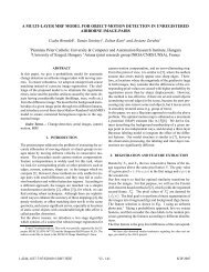
template observation proposed GMMREG CPD<br />
Fig. 1. Some results on the synthetic images. Observation and registered objects were overlayed, overlapping voxels are shown in yellow, while non-overlapping<br />
ones in red and green.<br />
size <strong>of</strong> the template object |F t | and the number <strong>of</strong> function<br />
calls I.<br />
As an example, we will now analyze the complexity <strong>of</strong><br />
a third order polynomial deformation (i.e. d = 3) model<br />
used also in our experiments. To generate sufficiently many<br />
equations, we need at least k = 60 ω i functions. Therefore let<br />
us choose power functions with maximal degree <strong>of</strong> 3:<br />
{(n i , m i , o i )} 64<br />
i=1 = {(a, b, c) | 0 ≤ a, b, c ≤ 3} (20)<br />
generating a total <strong>of</strong> 64 equations. Using the formulas above,<br />
64∑<br />
i=1<br />
d M = 33<br />
γ(d M ) = 7, 140<br />
γ(d i )γ(n i + m i + o i + 1) = 16, 453, 488<br />
In our experiments the average number <strong>of</strong> function calls was<br />
380 for this deformation model and ω i set. Note that the<br />
number <strong>of</strong> function calls is the same for both formulas, since<br />
they evaluate the same entity but in different ways. Hence, the
computational complexity <strong>of</strong> the formula (17) will be<br />
O(64|F o | + 7, 140|F t | + 380 · 16, 453, 488), (21)<br />
while the complexity <strong>of</strong> the original formula is<br />
O(64|F o | + 380(64 + 60 + 90)|F t |). (22)<br />
We thus conclude, that it is worth to use the formula (17)<br />
when<br />
|F t | ≥ 84, 286. (23)<br />
Runtime (min)<br />
δ(%)<br />
m µ σ m µ σ<br />
13.96 6.85 17.84 7.02 6.06 4.58<br />
TABLE I<br />
RESULTS ON 550 SYNTHETIC IMAGES (M – MEDIAN, µ – MEAN<br />
AND σ – STANDARD DEVIATION).<br />
transformed triangular mesh, from which the final voxelized<br />
object was obtained by the binvox program available from<br />
http://www.cs.princeton.edu/ ∼ min/binvox/ [13].<br />
Delta error (%)<br />
45<br />
40<br />
35<br />
30<br />
25<br />
20<br />
15<br />
10<br />
5<br />
0<br />
Proposed<br />
GMMREG 2.5<br />
GMMREG 4.5<br />
GMMREG 6.5<br />
CPD 4.5<br />
50 100 150 200<br />
Fig. 2. Comparison with GMMREG [1] and CPD [9].<br />
IV. EXPERIMENTAL RESULTS<br />
In our experiments, we used a third order polynomial<br />
deformation model (i.e. d = 3), which has a total <strong>of</strong> k =<br />
(d + 3)(d + 2)(d + 1)/2 = 60 parameters. A system <strong>of</strong> 64<br />
equations were generated by the set ω i (x) = x n i<br />
1 xm i<br />
2 xo i<br />
where {(n i , m i , o i )} 64<br />
i=1 = {(a, b, c) | 0 ≤ a, b, c ≤ 3}.<br />
The algorithm has been implemented in C++ using the<br />
levmar library written by M.I.A. Lourakis [12]. All tests<br />
were ran under a Linux system running on a virtualized<br />
Core i5 3.1 GHz architecture. The registration error has been<br />
quantitatively evaluated based on the absolute difference <strong>of</strong><br />
the aligned objects:<br />
3 ,<br />
δ = |F r △ F o | · 100%, (24)<br />
|F r | + |F o |<br />
where F o and F r denote the set <strong>of</strong> foreground voxels <strong>of</strong> the<br />
observation and registered objects respectively.<br />
In order to quantitatively evaluate the performance <strong>of</strong> the<br />
proposed method, a synthetic database <strong>of</strong> 500 deformed objects<br />
has been created. Observations have been generated by<br />
applying second and third order polynomial deformations to<br />
different template objects. The transformation parameters were<br />
randomly picked from the following intervals: a 11 , b 21 , c 31 ∈<br />
[0.5; 1.5], a 21 , a 31 , b 11 , b 31 , c 11 , c 21 ∈ [−0.25; 0.25] and all<br />
other parameters are from [−0.5; 0.5]. Note that a 00 = b 00 =<br />
c 00 = 0 (i.e. no translations), because initial normalization<br />
would remove any larger translations. Some <strong>of</strong> our results are<br />
presented in Fig. 1, where observation and registered objects<br />
were overlayed, overlapping voxels are shown in yellow, while<br />
non-overlapping ones in red and green. The statistics <strong>of</strong> our<br />
test are described in Table I.<br />
The registered objects, as well as synthetic observations,<br />
were generated by the following procedure (in Matlab): First,<br />
a smooth triangular mesh has been created from the object’s<br />
surface using Matlab’s internal isosurface function. Then<br />
the transformation was applied to the vertices yielding the<br />
We have compared our results to the point-based registration<br />
frameworks in [1] (GMMREG) and [9] (CPD). We used<br />
the C++ implementation <strong>of</strong> these methods available from<br />
http://code.google.com/p/gmmreg and set the parameters to<br />
their default values. At a first stage, we used all <strong>of</strong> the surface<br />
voxels as the input point set to the algorithm. For these<br />
sets consisting <strong>of</strong> about 0.5 megavoxel, the algorithms were<br />
running more than 12 hours without finding the transformation.<br />
Therefore the size <strong>of</strong> the point sets was reduced by using the<br />
vertices <strong>of</strong> an approximating triangular surface with various<br />
resolutions [14]. The mesh resolution was controlled by the<br />
maximal radius r <strong>of</strong> the corresponding Delaunay sphere. In<br />
Fig. 2, quantitative results for r = {2.5, 4.5, 6.5} indicate that<br />
these methods provide inferior alignments.<br />
In practice, segmentation never produces perfect shapes,<br />
therefore robustness against segmentation errors was also<br />
evaluated on simulated data: we randomly added or removed<br />
squares uniformly around the boundary <strong>of</strong> each slice <strong>of</strong> the<br />
observations yielding a surface error <strong>of</strong> 15%, 22% and 30%<br />
<strong>of</strong> the original object volume (see sample slices in Fig. 4).<br />
Fig. 3 shows the quantitative evaluation <strong>of</strong> the alignment error<br />
δ on more than 115 objects and the same test for the best<br />
GMMREG set (where r = 2.5). Considering that a δ < 10%<br />
corresponds to a visually good alignment, our approach is<br />
quite robust up to as high as 22% surface error.<br />
A. Medical application<br />
Lung alignment is a crucial task in lung cancer diagnosis<br />
[15]. During the treatment, changes in the tumor size<br />
are determined by comparing follow-up PET/CT scans which<br />
are taken at regular intervals depending on the treatment and<br />
the size <strong>of</strong> the tumor. Due to respiratory motion, the lung<br />
is subject to a nonlinear deformation between such followups,<br />
hence it is hard to automatically find correspondences.<br />
A common practice is to determine corresponding regions<br />
by hand, but this makes the procedure time consuming and
Delta errors (%)<br />
Delta errors (%)<br />
Delta errors (%)<br />
60<br />
50<br />
40<br />
30<br />
20<br />
10<br />
0<br />
60<br />
50<br />
40<br />
30<br />
20<br />
10<br />
0<br />
60<br />
50<br />
40<br />
30<br />
20<br />
10<br />
0<br />
Proposed<br />
GMMREG 2.5<br />
Proposed<br />
GMMREG 2.5<br />
Proposed<br />
GMMREG 2.5<br />
20 40 60 80 100<br />
15%<br />
20 40 60 80 100<br />
22%<br />
20 40 60 80 100<br />
30%<br />
Fig. 3. Robustness test comparison with the best GMMREG set (r = 2.5).<br />
original 15% 22% 30%<br />
Fig. 4.<br />
Sample surface errors on a slice.<br />
the obtained alignments may not be accurate enough for<br />
measuring changes.<br />
Our algorithm has been successfully applied to align <strong>3D</strong><br />
lung CT scans. The polynomial model proved to be a good approximation<br />
<strong>of</strong> the underlying physical deformation. Promising<br />
results were obtained on the available 8 image pairs with<br />
a median δ error <strong>of</strong> 8.41% (the mean and standard deviation<br />
were 7.99% and 3.03%, respectively). Some <strong>of</strong> these results<br />
are presented in Fig. 5, where we also show the achieved<br />
alignment on grayscale slices <strong>of</strong> the original lung CT images.<br />
For these slices, the original and transformed images were<br />
combined as an 8 × 8 checkerboard pattern.<br />
V. CONCLUSIONS<br />
We have proposed a novel elastic registration method which<br />
works without established correspondences. The basic idea<br />
is to set-up a system <strong>of</strong> non-linear equations whose solution<br />
directly provides the parameters <strong>of</strong> the aligning transformation.<br />
Herein, we considered a polynomial deformation model, but<br />
other diffeomorphism can also be used by approximating it<br />
via a Taylor expansion. The computational complexity has<br />
been analyzed for two alternative forms <strong>of</strong> the equations and<br />
optimal choice between these computational schemes has also<br />
been discussed. The efficiency and robustness <strong>of</strong> the proposed<br />
approach have been demonstrated on a large synthetic dataset.<br />
Our method compares favorably to two recent <strong>3D</strong> matching<br />
algorithms [1], [9]. Finally, the algorithm achieved promising<br />
results in aligning lung CT images.<br />
ACKNOWLEDGMENT<br />
This research was partially supported by the grant<br />
CNK80370 <strong>of</strong> the National Innovation Office (NIH) & the<br />
Hungarian Scientific Research Fund (OTKA); the European<br />
Union and co-financed by the European Regional Development<br />
Fund within the project TÁMOP-4.2.1/B-09/1/KONV-<br />
2010-0005. Lung images provided by Mediso Ltd., Budapest,<br />
Hungary.<br />
REFERENCES<br />
[1] B. Jian and B. C. Vemuri, “Robust point set registration using Gaussian<br />
mixture models,” IEEE Transactions on Pattern Analysis and Machine<br />
Intelligence, vol. 33, no. 8, pp. 1633–1645, Aug. 2011. [Online].<br />
Available: http://gmmreg.googlecode.com<br />
[2] C. Papazov and D. Burschka, “<strong>Deformable</strong> <strong>3D</strong> shape registration based<br />
on local similarity transforms,” Computer Graphics Forum, vol. 30,<br />
no. 5, pp. 1493–1502, Aug. 2011.<br />
[3] R. Sagawa, K. Akasaka, Y. Yagi, H. Hamer, and L. Van Gool, “<strong>Elastic</strong><br />
convolved ICP for the registration <strong>of</strong> deformable objects,” in Proceedings<br />
<strong>of</strong> International Conference on Computer Vision, IEEE. Kyoto,<br />
Japan: IEEE, Oct. 2009, pp. 1558–1565.<br />
[4] F. Michel, M. M. Bronstein, A. M. Bronstein, and N. Paragios, “Boosted<br />
metric learning for <strong>3D</strong> multi-modal deformable registration,” in Proceedings<br />
<strong>of</strong> International Symposium on Biomedical Imaging: From Nano to<br />
Macro, IEEE. Chicago, Illinois, USA: IEEE, Mar. 2011, pp. 1209–<br />
1214.<br />
[5] M. Holden, “A review <strong>of</strong> geometric transformations for nonrigid body<br />
registration,” IEEE Transactions on Medical Imaging, vol. 27, no. 1, pp.<br />
111–128, 2008.<br />
[6] F. L. Bookstein, “Principal warps: Thin-Plate Splines and the Decomposition<br />
<strong>of</strong> deformations,” IEEE Transactions on Pattern Analysis and<br />
Machine Intelligence, vol. 11, no. 6, pp. 567–585, 1989.
Fig. 5.<br />
Alignment <strong>of</strong> lung CT volumes. Segmented <strong>3D</strong> lung images were generated by the InterView Fusion s<strong>of</strong>tware <strong>of</strong> Mediso Ltd.<br />
[7] L. Zagorchev and A. Goshtasby, “A comparative study <strong>of</strong> transformation<br />
functions for nonrigid image registration,” IEEE Transactions on Image<br />
Processing, vol. 15, no. 3, pp. 529 –538, march 2006.<br />
[8] C. Domokos, J. Nemeth, and Z. Kato, “Nonlinear Shape <strong>Registration</strong><br />
without Correspondences,” IEEE Transactions on Pattern Analysis and<br />
Machine Intelligence, vol. 34, no. 5, pp. 943–958, 2012.<br />
[9] A. Myronenko, X. B. Song, and M. Á. Carreira-Perpiñán, “Non-rigid<br />
point set registration: Coherent point drift,” in Proceedings <strong>of</strong> the Annual<br />
Conference on Neural Information Processing Systems, B. Schölkopf,<br />
J. C. Platt, and T. H<strong>of</strong>fman, Eds. Vancouver, British Columbia, Canada:<br />
MIT Press, Dec. 2006, pp. 1009–1016.<br />
[10] S. Belongie, J. Malik, and J. Puzicha, “Shape matching and object<br />
recognition using shape context,” IEEE Transactions on Pattern Analysis<br />
and Machine Intelligence, vol. 24, no. 4, pp. 509–522, April 2002.<br />
[11] R. Merris, Combinatorics, ser. Wiley Series in Discrete Mathematics<br />
and Optimization. John Wiley, 2003. [Online]. Available: http:<br />
//books.google.hu/books?id=OM3CP4i58b4C<br />
[12] M. Lourakis, “levmar: Levenberg-marquardt nonlinear least squares<br />
algorithms in C/C++,” [web page] http://www.ics.forth.gr/ ∼ lourakis/<br />
levmar/, Jul. 2004, [Accessed on 14 Jun. 2012.].<br />
[13] F. S. Nooruddin and G. Turk, “Simplification and repair <strong>of</strong> polygonal<br />
models using volumetric techniques,” IEEE Transactions on Visualization<br />
and Computer Graphics, vol. 9, no. 2, pp. 191 – 205, Apr. 2003.<br />
[14] Q. Fang and D. Boas, “Tetrahedral mesh generation from volumetric<br />
binary and gray-scale images,” in Proceedings <strong>of</strong> International Symposium<br />
on Biomedical Imaging: From Nano to Macro, IEEE. Boston,<br />
Massachusetts, USA: IEEE, Jun. 2009, pp. 1142–1145.<br />
[15] A. S. Bryant and R. J. Cerfolio, “The maximum standardized<br />
uptake values on integrated FDG-PET/CT is useful in differentiating<br />
benign from malignant pulmonary nodules,” The Annals <strong>of</strong> Thoracic<br />
Surgery, vol. 82, pp. 1016–1020, 2006. [Online]. Available: http:<br />
//ats.ctsnetjournals.org/cgi/content/abstract/82/3/1016