Unsupervised Recursive Sequence Processing - Institute of ...

Unsupervised Recursive Sequence Processing
Marc Strickert, Barbara Hammer
Research group LNM, Department of Mathematics/Computer Science,
University of Osnabrück, Germany
Sebastian Blohm
Institute for Cognitive Science,
University of Osnabrück, Germany
Abstract
The self organizing map (SOM) is a valuable tool for data visualization and data mining for
potentially high dimensional data of an a priori fixed dimensionality. We investigate SOMs
for sequences and propose the SOM-S architecture for sequential data. Sequences of potentially
infinite length are recursively processed by integrating the currently presented item
and the recent map activation, as proposed in [11]. We combine that approach with the
hyperbolic neighborhood of Ritter [29], in order to account for the representation of possibly
exponentially increasing sequence diversification over time. Discrete and real-valued
sequences can be processed efficiently with this method, as we will show in experiments.
Temporal dependencies can be reliably extracted from a trained SOM. U-Matrix methods,
adapted to sequence processing SOMs, allow the detection of clusters also for real-valued
sequence elements.
Key words: Self-organizing map, sequence processing, recurrent models, hyperbolic
SOM, U-Matrix, Markov models
1 Introduction
Unsupervised clustering by means of the self organizing map (SOM) was first proposed
by Kohonen [21]. The SOM makes the exploration of high dimensional data
possible and it allows the exploration of the topological data structure. By SOM
training, the data space is mapped to a typically two dimensional Euclidean grid
Email address: {marc,hammer}@informatik.uni-osnabrueck.de
(Marc Strickert, Barbara Hammer).
Preprint submitted to Elsevier Science 23 January 2004

of neurons, preferably in a topology preserving manner. Prominent applications of
the SOM are WEBSOM for the retrieval of text documents and PicSOM for the
recovery and ordering of pictures [18,25]. Various alternatives and extensions to
the standard SOM exist, such as statistical models, growing networks, alternative
lattice structures, or adaptive metrics [3,4,19,27,28,30,33].
If temporal or spatial data are dealt with – like time series, language data, or DNA
strings – sequences of potentially unrestricted length constitute a natural domain for
data analysis and classification. Unfortunately, the temporal scope is unknown in
most cases, and therefore fixed vector dimensions, as used for standard SOM, cannot
be applied. Several extensions of SOM to sequences have been proposed; for
instance, time-window techniques or the data representation by statistical features
make a processing with standard methods possible [21,28]. Due to data selection or
preprocessing, information might get lost; for this reason, a data-driven adaptation
of the metric or the grid is strongly advisable [29,33,36]. The first widely used application
of SOM in sequence processing employed the temporal trajectory of the
best matching units of a standard SOM in order to visualize speech signals and the
variations of which [20]. This approach, however, does not operate on sequences
as they are; rather, SOM is used for reducing the dimensionality of single sequence
entries and acts as a preprocessing mechanism this way. Proposed alternatives substitute
the standard Euclidean metric by similarity operators on sequences by incorporating
autoregressive processes or time warping strategies [16,26,34]. These
methods are very powerful, but a major problem is their computational costs.
A fundamental way for sequence processing is a recursive approach. Supervised
recurrent networks constitute a well-established generalization of standard feedforward
networks to time series; many successful applications for different sequence
classification and regression tasks are known [12,24]. Recurrent unsupervised models
have also been proposed: the temporal Kohonen map (TKM) and the recurrent
SOM (RSOM) use the biologically plausible dynamics of leaky integrators [8,39],
as they occur in organisms, and explain phenomena such as direction selectivity
in the visual cortex [9]. Furthermore, the models have been applied with moderate
success to learning tasks [22]. Better results have been achieved by integrating these
models into more complex systems [7,17]. Recent more powerful approaches are
the recursive SOM (RecSOM) and the SOM for structured data (SOMSD) [10,41].
These are based on a richer and explicit representation of the temporal context: they
use the activation profile of the entire map or the index of the most recent winner.
As a result, their representation ability is superior to RSOM and TKM.
A proposal to put existing unsupervised recursive models into a taxonomy can be
found in [1,2]. The latter article identifies the entity ’time context’ used by the models
as one of the main branches of the given taxonomy [2]. Although more general,
the models are still quite diverse, and the recent developments of [10,11,35] are
not included in the taxonomy. An earlier, simple, and elegant general description of
recurrent models with an explicit notion of context has been introduced in [13,14].
2

This framework directly generalizes the dynamics of supervised recurrent networks
to unsupervised models and it contains TKM, RecSOM, and SOMSD as special
cases. As pointed out in [15], the precise approaches differ with respect to the
notion of context and therefore they yield different accuracies and computational
complexities, but their basic dynamic is the same. TKM is restricted due to the
locality of its context representation, whereas RecSOM and SOMSD also include
global information. In that regard, SOMSD can be interpreted as a modification
of RecSOM, based on a compression of the RecSOM context model, and being
computationally less demanding. Alternative efficient compression schemes such
as Merging SOM (MSOM) have recently been developed [37].
Here, we will focus on the compact and flexible representation of time context
by linking the current winner neuron to the most recently presented sequence element:
a neuron’s temporal context is given by an explicit back-reference to the best
matching unit of the past time step, representing the previously processed input as
the location of the last winning neuron in the map, as proposed in [10]. In comparison
to RecSOM, this yields a greatly reduced computation time: the context of
SOMSD is a low-dimensional (usually two-dimensional) vector compared to a N-
dimensional vector of RecSOM, N being the number of neurons (usually, N is at
least 100). In addition, the explicit reference to the past winning unit allows elegant
ways for extracting temporal dependencies. We will show how Markov models can
be easily obtained from a trained map. This is not only possible for discrete input
symbols, but also for real-valued sequence entries, by applying an adaptation
of standard U-Matrix methods [38] to recursive SOMs. We will demonstrate the
faithful representation of several time series and Markov processes within SOMSD
in this article. However, SOMSD heavily relies on an adequate grid topology, because
the distance of context representations is measured within the grid structure.
It can be expected that low dimensional regular lattices do not capture typical
characteristics of the space of time series. For this reason, we extend the SOMSD
approach to more general topologies, that is to possibly non-Euclidean triangular
grid structures. In particular, we combine a hyperbolic grid and the last-winner-ingrid
temporal back reference. Hyperbolic grid structures have been proposed and
successfully applied to document organization and retrieval [29,30]. Unlike rectangular
lattices with inherent power law neighborhood growth, HSOM implements
an exponential neighborhood growth. For discrete and real-valued time series we
will evaluate the combination of hyperbolic lattices with the recurrent dynamics,
putting the focus on neuron specialization, activations, and weight distributions.
First, we present some recursive self-organizing map models introduced in the literature,
which use different notions of context. Then, we explain the SOM for structured
data (SOMSD) adapted to sequences in detail, and we extend the model to
arbitrary triangular grid structures. After that, we propose an algorithm to extract
Markov models from a trained map and we show how this algorithm can be combined
with U-Matrix methods. Finally, we demonstrate in experiments the sequence
representation capabilities, using several discrete and real-valued benchmark series.
3

2 Unsupervised processing of sequences
Let input sequences be denoted by s = (s 1 , . . . , s t ) with entries s i in an alphabet
Σ which is embedded in a real-vector space R n . The element s 1 denotes the most
recent entry of the sequence and t is the sequence length.The set of sequences of
arbitrary length over symbols Σ is Σ ∗ , and Σ l is the space of sequences of length l.
Popular recursive sequence processing models are the temporal Kohonen map,
recurrent SOM, recursive SOM, and SOM for structured data [8,11,39,41]. The
SOMSD has originally been proposed for the more general case of tree structure
processing. Here, only sequences, i.e. trees with a node fan-out of 1 are considered.
As for standard SOM, a recursive neural map is given by a set of neurons n 1 , . . . ,
n N . The neurons are arranged on a grid, often a two-dimensional regular lattice.
All neurons are equipped with weights w i ∈ R n .
Two important ingredients have to be defined to specify self-organizing network
models: the data metric and the network update. The metric addressed the question,
how an appropriate distance can be defined to measure the similarity of possibly
sequential input signals to map units. For this purpose, the sequence entries
are compared with the weight parameters stored at the neuron. The set of input signals
for which a given neuron i is closest, is called the receptive field of neuron i,
and neuron i is the winner and representative for all these signals within its receptive
field. In the following, we will recall the distance computation for the standard
SOM and also review several ways found in the literature to compute the distance
of a neuron from a sequential input. Apart from the metric, the update procedure or
learning rule for neurons to adapt to the input is essential. Commonly, Hebbian or
competitive 1 learning takes place, referring to the following scheme: the parameters
of the winner and its neighborhood within a given lattice structure are adapted
such that their response to the current signal is increased. Thereby, neighborhood
cooperation ensures a topologically faithful mapping.
Standard SOM relies on a simple winner-takes-all scheme and does not account
for the temporal structure of inputs. For a stimulus s i ∈ R n the neuron n j responds,
for which the squared distance
d SOM (s i , w j ) = ‖s i − w j ‖ 2 ,
s i ∈ R n
is minimum, where ‖ · ‖ is the standard Euclidean metric. Training starts with
randomly initialized weights w i and adapts the parameters iteratively as follows:
denote by n 0 the index of the winning neuron for the input signal s i . Assume a
function nhd(n j , n k ) which indicates the degree of neighborhood of neuron j and
k within the chosen lattice structure is fixed. Adaptation of all weights w j takes
1 We will use these two terms interchangeably in the following.
4

place by the update rule
△w j = ɛ · h σ (nhd(n j0 , n j )) · (s i − w j )
whereby ɛ ∈ (0, 1) is the learning rate. The function h σ describes the amount of
neuron adaptation in the neighborhood of the winner: often the Gaussian bell function
h σ (x) = exp(−x 2 /σ 2 ) is chosen, of which the shape is narrowed during training
by decreasing σ to ensure the neuron specialization. The function nhd(n j , n k )
which measures the degree of neighborhood of the neurons n i and n j within the
lattice might be induced by the simple Euclidean distance between the neuron coordinates
in a rectangular grid or by the shortest distance in a graph connecting the
two neurons.
Recursive models substitute the one-shot distance computation for a single entry
s i by a recursive formula over all entries of a given sequence s. For all models,
sequences are presented recursively, and the current sequence entry s i is processed
in the context which is set by its predecessors s i+1 , s i+2 , . . .. 2 The models differ
with respect to the representation of the context and in the way that the context
influences further computation.
The Temporal Kohonen Map (TKM) computes the distance of s = (s 1 , . . . , s t )
from neuron n j labeled with w j ∈ R n by the leaky integration
t∑
d TKM (s, n j ) = η(1 − η) i−1 ‖s i − w j ‖ 2
i=1
where η ∈ (0, 1) is a memory parameter [8]. A neuron becomes winner if the
current entry s 1 is close to its weight w j as in standard SOM, and, in addition,
the remaining sum (1 − η)‖s 2 − w j ‖ + (1 − η) 2 ‖s 3 − w j ‖ + . . . is also small.
This additional term integrates the distances of the neuron’s weight from previous
sequence entries weighted by an exponentially decreasing decay factor (1 − η) i−1 .
The context resulting from previous sequence entries is pointing towards neurons
of which the weights have been close to previous entries. Thus, the winner is a
neuron whose weight is close to the average presented signal for the recent time
steps.
The training for the TKM takes place by Hebbian learning in the same way as for
the standard SOM, making well-matching neurons more similar to the current input
than bad-matching neurons. At the beginning, weights w j are initialized randomly
and then iteratively adapted when data is presented. For adaptation assume that a
2 We use reverse indexing of the sequence entries, s 1 denoting the most recent entry,
s 2 , s 3 , . . . its predecessors.
5

sequence s is given, with s i denoting the current entry and n j0 denoting the best
matching neuron for this time step. Then the weight correction term is
△w j = ɛ · h σ (nhd(n j0 , n j )) · (s i − w j )
As discussed in [23], the learning rule of TKM is unstable and leads to only suboptimal
results. More advanced, the Recurrent SOM (RSOM) leaky integration first
sums up the weighted directions and afterwards computes the distance [39]
t∑
2
d RSOM (s, n j ) =
η(1 − η) i−1 (s
∥
i − w j )
.
∥
i=1
It represents the context in a larger space than TKM since the vectors of directions
are stored instead of the scalar Euclidean distance. More importantly, the training
rule is changed. RSOM derives its learning rule directly from the objective to minimize
the distortion error on sequences and thus adapts the weights towards the
vector of integrated directions:
△w j = ɛ · h σ (nhd(n j0 , n j )) · y j (i)
whereby
y j (i) =
t∑
η(1 − η) i−1 (s i − w j ) .
i=1
Again, the already processed part of the sequence produces a context notion, and
the neuron becomes the winner for the current entry of which the weight is most
similar to the average entry for the past time steps. The training rule of RSOM takes
this fact into account by adapting the weights towards this averaged activation.
We will not refer to this learning rule in the following. Instead, the way in which
sequences are represented within these two models, and the ways to improve the
representational capabilities of such maps will be of interest.
Assuming vanishing neighborhood influences σ for both cases TKM and RSOM,
one can analytically compute the internal representation of sequences for these two
models, i.e. weights with response optimum to a given sequence s = (s 1 , . . . , s t ):
the weight w is optimum for which
t∑
t∑
w = (1 − η) i−1 s i / (1 − η) i−1
i=1
i=1
holds [40]. This explains the encoding scheme of the winner-takes-all dynamics
of TKM and RSOM. Sequences are encoded in the weight space by providing a
6

ecursive partitioning very much like the one generating fractal Cantor sets. As an
example for explaining this encoding scheme, assume that binary sequences {0, 1} l
are dealt with. For η = 0.5, the representation of sequences of fixed length l corresponds
to an encoding in a Cantor set: the interval [0, 0.5) represents sequences
with most recent entry s 1 = 0, interval [0.5, 1) contains only codes of sequences
with most recent entry 1. Recursive decomposition of the intervals allows to recover
further entries of the sequence: [0, 0.25) stands for the beginning 00. . . of a
sequence, [0.25, 0.5) stands for 01, [0.5, 0.75) for 10, and [0.75, 1) represents 11.
By further subdivision, [0, 0.125) stands for the beginning 000. . ., [0.125, 0.25) for
001, and so on. Similar encodings can be found for alternative choices of η. Sequences
over discrete sets Σ = {0, . . . , d} ⊂ R can be uniquely encoded using
this fractal partitioning if η < 1/d. For larger η, the subsets start to overlap, i.e.
codes are no longer sorted according to their last symbols, and a code might stand
for two or more different sequences. A very small η ≪ 1/d, in turn, results in an
only sparsely used space; for example the interval (d · η, 1] does not contain a valid
code. Note that the explicit computation of this encoding stresses the superiority
of the RSOM learning rule compared to TKM update, as pointed out in [40]: the
fractal code is a fixed point for the dynamics of RSOM training, whereas TKM
converges towards the borders of the intervals, preventing the optimum fractal encoding
scheme from developing on its own.
Fractal encoding is reasonable, but limited: it is obviously restricted to discrete
sequence entries, and real values or noise might destroy the encoded information.
Fractal codes do not differentiate between sequences of different length; e.g. the
code 0 gives optimum response to 0,00, 000, and so forth. Sequences with this
kind of encoding cannot be distinguished. In addition, the number of neurons does
not take influence on the expressiveness of the context space. The range in which
sequences are encoded is the same as the weight space. Thus, both the size of the
weight space and the computation accuracy are limiting the number of different
contexts, independently of the number of neurons of the network.
Based on these considerations, richer and in particular explicit representations of
context have been proposed. The models that we introduce in the following extend
the parameter space of each neuron j by an additional vector c j , which is
used to explicitly store the sequential context within which a sequence entry is expected.
Depending on the model, the context c j is contained in a representation
space with different dimensionality. However, in all cases this space is independent
of the weight space and extends the expressiveness of the models in comparison
to TKM and RSOM. For each model, we will define the basic ingredients: what is
the space of context representations? How is the distance between a sequence entry
and neuron j computed, taking into account its temporal context c j ? How are the
weights and contexts adapted?
The Recursive SOM (RecSOM) [41] equips each neuron n j with a weight w j ∈
R n that represents the given sequence entry, as usual. In addition, a vector c j ∈
7

R N is provided, N denoting the number of neurons, which explicitly represents
the contextual map activation of all neurons in the previous time step. Thus, the
temporal context is represented in this model in an N-dimensional vector space, N
denoting the number of neurons. One can think of the context as an explicit storage
of the activity profile of the whole map in the previous time step. More precisely,
distance is recursively computed by
d RecSOM ((s 1 , . . . , s t ), n j ) = η 1 ‖s 1 − w j ‖ 2 + η 2 ‖C RecSOM (s 2 , . . . , s t ) − c j ‖ 2
where η 1 , η 2 > 0.
C RecSOM (s) = (exp(−d RecSOM (s, n 1 )), . . . , exp(−d RecSOM (s, n N )))
constitutes the context. Note that this vector is almost the vector of distances of all
neurons computed in the previous time step. These are exponentially transformed
to avoid an explosion of the values. As before, the above distance can be decomposed
into two parts: the winner computation similar to standard SOM, and, as in
the case of RSOM and TKM, a term which assesses the context match. For Rec-
SOM the context match is a comparison of the current context when processing
the sequence, i.e. the vector of distances of the previous time step, and the expected
context c j which is stored at neuron j. That is to say, RecSOM explicitly stores context
vectors for each neuron and compares these context vectors to their expected
contexts during the recursive computation. Since the entire map activation is taken
into account, sequences of any given fixed length can be stored, if enough neurons
are provided. Thus, the representation space for context is no longer restricted by
the weight space and its capacity now scales with the number of neurons.
For RecSOM, training is done in Hebbian style for both weights and contexts. Denote
by n j0 the winner for sequence entry i, then the weight changes are
△w j = ɛ · h σ (nhd(n j0 , n j )) · (s i − w j )
and the context adaptation is
△c j = ɛ ′ · h σ (nhd(n j0 , n j )) · (C RecSOM (s i+1 , . . . , s t ) − c j )
The latter update rule makes sure that the context vectors of the winner neuron
and its neighborhood become more similar to the current context vector C RecSOM ,
which is computed when the sequence is processed. The learning rates are ɛ, ɛ ′ ∈
(0, 1). As demonstrated in [41], this richer representation of context allows a better
quantization of time series data. In [41], various quantitative measures to evaluate
trained recursive maps are proposed, such as the temporal quantization error and
the specialization of neurons. RecSOM turns out to be clearly superior to TKM and
RSOM with respect to these measures in the experiments provided in [41].
8

However, the dimensionality of the context for RecSOM equals the number of neurons
N, making this approach computationally quite costly. The training of very
huge maps with several thousands of neurons is no longer feasible for RecSOM.
Another drawback is given by the exponential activity transfer function in the term
of C RecSOM ∈ R N : specialized neurons are characterized by the fact that they have
only one or a few well-matching predecessors contributing values of about 1 to
C RecSOM ; however, for a large number N of neurons, the noise influence on C RecSOM
from other neurons destroys the valid context information, because even poorly
matching neurons – contributing values of slightly above 0 – are summed up in the
distance computation.
SOM for structured data (SOMSD) as proposed in [10,11] is an efficient and still
powerful alternative. SOMSD represents temporal context by the corresponding
winner index in the previous time step. Assume that a regular l-dimensional lattice
of neurons is given. Each neuron n j is equipped with a weight w j ∈ R n and a
value c j ∈ R l which represents a compressed version of the context, the location
of the previous winner within the map [10]. The space in which context vectors
are represented is the vector space R l for this model. The distance of sequence
s = (s 1 , . . . , s t ) from neuron n j is recursively computed by
d SOMSD ((s 1 , . . . , s t ), n j ) = η 1 ‖s 1 − w j ‖ 2 + η 2 ‖C SOMSD (s 2 , . . . , s n ) − c j ‖ 2
where C SOMSD (s) equals the location of neuron n j with smallest d SOMSD (s, n j ) in the
grid topology. Note that the context C SOMSD is an element in a low-dimensional vector
space, usually only R 2 . The distance between contexts is given by the Euclidean
metric within this vector space. The learning dynamic of SOMSD is very similar
to the dynamic of RecSOM: the current distance is defined as a mixture of two
terms, the match of the neuron’s weight and the current sequence entry, and the
match of the neuron’s context weight and the context currently computed in the
model. Thereby, the current context is represented by the location of the winning
neuron of the map in the previous time step. This dynamic imposes a temporal bias
towards those neurons which context vector matches the winner location of the previous
time step. It relies on the fact that a lattice structure of neurons is defined and
a distance measure of locations within the map is defined.
Due to the compressed context information, this approach is very efficient in comparison
to RecSOM and also very large maps can be trained. In addition, noise
is suppressed in this compact representation. However, more complex context information
is used than for TKM and RSOM, namely the location of the previous
winner in the map. As for RecSOM, Hebbian learning takes place for SOMSD, because
weight vectors and contexts are adapted in a well-known correction manner,
here by the formulas
△w j = ɛ · h σ (nhd(n j0 , n j )) · (s i − w j )
9

and
△c j = ɛ ′ · h σ (nhd(n j0 , n j )) · (C SOMSD (s i+1 , . . . , s t ) − c j )
with learning rates ɛ, ɛ ′ ∈ (0, 1). n j0 denotes the winner for sequence entry i.
As demonstrated in [11], a generalization of this approach to tree structures can
reliably model structured objects and their respective topological ordering.
We would like to point out that, although these approaches seem different, they
constitute instances of the same recursive computation scheme. As proved in [14],
the underlying recursive update dynamics comply with
d((s 1 , . . . , s t ), n j ) = η 1 ‖s 1 − w j ‖ 2 + η 2 ‖C(s 2 , . . . , s n ) − c j ‖ 2
in all the cases. Their specific similarity measures for weights and contexts are denoted
by the generic ‖ · ‖ expression. The approaches differ with respect to the
concrete choice of the context C: TKM and RSOM refer to only the neuron itself
and are therefore restricted to local fractal codes within the weight space; RecSOM
uses the whole map activation, which is powerful but also expensive and subject
to random neuron activations; SOMSD relies on compressed information, the location
of the winner. Note that also standard supervised recurrent networks can be
put into the generic dynamic framework by choosing the context as the output of
the sigmoidal transfer function [14]. In addition, alternative compression schemes,
such as a representation of the context by the winner content, are possible [37].
To summarize this section, essentially four different models have been proposed
for processing temporal information. The models are characterized by the way in
which context is taken into account within the map. The models are:
Standard SOM: no context representation; standard distance computation; standard
competitive learning.
TKM and RSOM: no explicit context representation; the distance computation
recursively refers to the distance of the previous time step; competitive learning
for the weight whereby (for RSOM) the averaged signal is used.
RecSOM: explicit context representation as N-dimensional activity profile of the
previous time step; the distance computation is given as mixture of the current
match and the match of the context stored at the neuron and the (recursively computed)
current context given by the processed time series; competitive learning
adapts the weight and context vectors.
SOMSD: explicit context representation as low-dimensional vector, the location
of the previously winning neuron in the map; the distance is computed recursively
the same way as for RecSOM, whereby a distance measure for locations
in the map has to be provided; so far, the model is only available for standard
rectangular Euclidean lattices; competitive learning adapts the weight and context
vectors, whereby the context vectors are embedded in the Euclidean space.
10

In the following, we focus on the context representation by the winner index, as
proposed in SOMSD. This scheme offers a compact and efficient context representation.
However, it relies heavily on the neighborhood structure of the neurons,
and faithful topological ordering is essential for appropriate processing. Since for
sequential data, like for words in Σ ∗ , the number of possible strings is an exponential
function of their length, an Euclidean target grid with inherent power law
neighborhood growth is not suited for a topology preserving representation. The
reason for this is that the storage of temporal data is related to the representation
of trajectories on the neural grid. String processing means beginning at a node that
represents the start symbol; then, how many nodes n s can in the ideal case uniquely
be reached in a fixed number s of steps? In grids with 6 neurons per neighbor the
triangular tessellation of the Euclidean plane leads to a hexagonal superstructure,
inducing the surprising answer of n s = 6 for any choice of s > 0. Providing 7
neurons per neighbor yields the exponential branching n s = 7 · 2 (s−1) of paths.
In this respect, it is interesting to note that RecSOM can also be combined with
alternative lattice structures; in [41] a comparison is presented of RecSOM with a
standard rectangular topology and a data optimum topology provided by neural gas
(NG) [27,28]. The latter clearly leads to superior results. Unfortunately, it is not
possible to combine the optimum topology of NG with SOMSD: for NG, no grid
with straightforward neuron indexing exists. Therefore, context cannot be defined
easily by referring back to the previous winner, because no similarity measure is
available for indices of neurons within a grid topology.
Here, we extend SOMSD to grid structures with triangular grid connectivity in
order to obtain a larger flexibility for the lattice design. Apart from the standard
Euclidean plane, the sphere and the hyperbolic plane are alternative popular twodimensional
manifolds. They differ from the Euclidean plane with respect to their
curvature: the Euclidean plane is flat, whereas the hyperbolic space has negative
curvature, and the sphere is curved positively. By computing the Euler characteristics
of all compact connected surfaces, it can be shown that only seven have nonnegative
curvature, implying that all but seven are locally isometric to the hyperbolic
plane, which makes the study of hyperbolic spaces particularly interesting. 3
The curvature has consequences on regular tessellations of the referred manifolds as
pointed out in [30]: the number of neighbors of a grid point in a regular tessellation
of the Euclidean plane follows a power law, whereas the hyperbolic plane allows
an exponential increase of the number of neighbors. The sphere yields compact
lattices with vanishing neighborhoods, whereby a regular tessellation for which all
vertices have the same number of neighbors is impossible (with the uninteresting
exception of an approximation by one of the 5 Platonic solids). Since all these
surfaces constitute two-dimensional manifolds, they can be approximated locally
within a cell of the tessellation by a subset of the standard Euclidean plane without
3 For an excellent tool box and introduction to hyperbolic geometry see e.g.
http://www.geom.uiuc.edu/docs/forum/hype/hype.html
11

too much contortion. A global isometric embedding, however, is not possible in
general. Interestingly, for all such tessellations a data similarity measure is defined
and possibly non-isometric visualization in the 2D plane can be achieved. While 6
neighbors per neuron lead to standard Euclidean triangular meshes, for a grid with
7 neighbors or more, the graph becomes part of the 2-dimensional hyperbolic plane.
As already mentioned, exponential neighborhood growth is possible and hence an
adequate data representation can be expected for the visualization of domains with
a high connectivity of the involved objects. SOM with hyperbolic neighborhood
(HSOM) has already proved well-suited for text representation as demonstrated for
a non-recursive model in [29].
3 SOM for sequences (SOM-S)
In the following, we introduce the adaptation of SOMSD for sequences and the
general triangular grid structure, SOM for sequences (SOM-S). Standard SOMs
operate on a rectangular neuron grid embedded in a real-valued vector space. More
flexibility for the topological setup can be obtained by describing the grid in terms
of a graph: neural connections are realized by assigning each neuron a set of direct
neighbors. The distance of two neurons is given by the length of a shortest path
within the lattice of neurons. Each edge is assigned the unit length 1. The number of
neighbors might vary (also within a single map). Less than 6 neighbors per neuron
lead to a subsiding neighborhood, resulting in graphs with small numbers of nodes.
Choosing more than 6 neighbors per neuron yields, as argued above, an exponential
increase of the neighborhood size, which is convenient for representing sequences
with potentially exponential context diversification.
Unlike standard SOM or HSOM, we do not assume that a distance preserving embedding
of the lattice into the two dimensional plane or another globally parameterized
two-dimensional manifold with global metric structure, such as the hyperbolic
plane, exists. Rather, we assume that the distance of neurons within the grid
is computed directly on the neighborhood graph, which might be obtained by any
non-overlapping triangulation of the topological two-dimensional plane. 4 For our
experiments, we have implemented a grid generator for a circular triangle meshing
around a center neuron, which requires the desired number of neurons and the
neighborhood degree n as parameters. Neurons at the lattice edge possess less than
n neighbors, and if the chosen total number of neurons does not lead to filling up
the outer neuron circle, neurons there are connected to others in a maximum symmetric
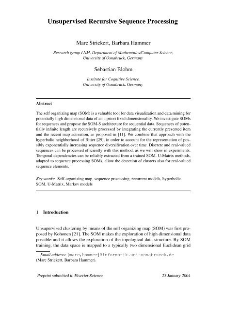
way. Figure 1 shows a small map with 7 neighbors for the inner neurons,
and a total of 29 neurons perfectly filling up the outer edge. For ≥ 7 neighbors, the
exponential neighborhood increase can be observed, for which an embedding into
4 Since the lattice is fixed during training, these values have to be computed only once.
12

,
!
!
,
Fig. 1. Hyperbolic self organizing map with context. Neuron n refers to the context given
by the winner location in the map, indicated by the triangle of neurons N 1 , N 2 , and N 3 ,
and the precise coordinates ß 12 ,ß 13 . If the previous winner has been D 2 , adaptation of the
context along the dotted line takes place.
the Euclidean plane is not possible without contortions; however, local projections
in terms of a fish eye magnification focus can be obtained (cf. [29]).
SOMSD adapts the location of the expected previous winner during training. For
this purpose, we have to embed the triangular mesh structure into a continuous
space. We achieve this by computing lattice distances beforehand, and then we approximate
the distance of points within a triangle shaped map patch by the standard
Euclidean distance. Thus, positions in the lattice are represented by three neuron
indices which represent the selected triangle of adjacent neurons, and two real numbers
which represent the position within the triangle. The recursive nature of the
shown map is illustrated exemplarily in figure 1 for neuron n. This neuron n is
equipped with a weight w ∈ R n and a context c that is given by a location within
the triangle of neurons N 1 , N 2 , and N 3 expressing corner affinities by means of
the linear combination parameters ß 12 and ß 13 . The distance of a sequence s from
neuron n is recursively computed by
d SOM-S ((s 1 , . . . , s t ), n) = η ‖s 1 − w‖ 2 + (1 − η) g(C SOM-S (s 2 , . . . , s n ), c).
C SOM-S (s) is the index of the neuron n j in the grid with smallest distance d SOM-S (s, n j ).
g measures the grid distance of the triangular position c j = (N 1 , N 2 , N 3 , ß 12 , ß 13 )
to the winner as the shortest possible path in the mesh structure. Grid distances
between neighboring neurons possess unit length, and the metric structure within
the triangle N 1 , N 2 , N 3 is approximated by the Euclidean metric. The range of g
is normalized by scaling with the inverse maximum grid distance. This mixture of
hyperbolic grid distance and Euclidean distance is valid, because the hyperbolic
space can locally be approximated by Euclidean space, which is applied for computational
convenience to both distance calculation and update.
13

Training is carried out by presenting a pattern s = (s 1 , . . . , s t ), determining the
winner n j0 , and updating the weight and the context. Adaptation affects all neurons
on the breadth first search graph around the winning neuron according to their
grid distances in a Hebbian style. Hence, for the sequence entry s i , weight w j is
updated by △w j = ɛ · h σ (nhd(n j0 , n j )) · (s i − w j ). The learning rate ɛ is typically
exponentially decreased during training; as above, h σ (nhd(n j0 , n j )) describes the
influence of the winner n j0 to the current neuron n j as a decreasing function of
grid distance. The context update is analogous: the current context, expressed in
terms of neuron triangle corners and coordinates, is moved towards the previous
winner along a shortest path. This adaptation yields positions on the grid only.
Intermediate positions can be achieved by interpolation: if two neurons N i and N j
exist in the triangle with the same distance, the midway is taken for the flat grids
obtained by our grid generator. This explains why the update path, depicted as the
dotted line in figure 1, for the current context towards D 2 is via D 1 . Since the grid
distances are stored in a static matrix, a fast calculation of shortest path lengths is
possible. The parameter η in the recursive distance calculations controls the balance
between pattern and context influence; since initially nothing is known about the
temporal structure, this parameter starts at 1, thus indicating the absence of context,
and resulting in standard SOM. During training it is decreased to an application
dependent value that mediates the balance between the externally presented pattern
and the internally gained model about historic contexts.
Thus, we can combine the flexibility of general triangular and possibly hyperbolic
lattice structures with the efficient context representation as proposed in [11].
4 Evaluation measures of SOM
Popular methods to evaluate the standard SOM are the visual inspection, the identification
of meaningful clusters, the quantization error, and measures for topological
ordering of the map. For recursive self organizing maps, an additional dimension
arises: the temporal dynamic stored in the context representations of the map.
4.1 Temporal quantization error
Using ideas of Voegtlin [41] we introduce a method to assess the implicit representation
of temporal dependencies in the map, and to evaluate to which amount
faithful representation of the temporal data takes place. The general quantization
error refers to the distortion of each map unit with respect to its receptive field,
which measures the extent of data space coverage by the units. If temporal data are
considered, the distortion needs to be assessed back in time. For a formal definition,
assume that a time series (s 1 , s 2 , . . . , s t , . . .) is presented to the network, again
14

with reverse indexing notation, i.e. s 1 is the most recent entry of the time series. Let
win i denote all time steps for which neuron i becomes the winner in the considered
recursive map model. The mean activation of neuron i for time step t in the past is
the value
A i (t) =
∑
s j+t /|win i |.
j∈win i
Assume that neuron i becomes winner for a sequence entry s j . It can then be expected
that s j is like the standard SOM close to the average A i (0), because the map
is trained with Hebbian learning. Temporal specification takes place if, in addition,
s j+t is close to the average A i (t) for t > 0. The temporal quantization error of
neuron i at time step t back in the past is defined by
⎛
⎞
E i (t) = ⎝ ∑
‖s j+t − A i (t)‖ 2 ⎠
j∈win i
1/2
.
This measures the extent up to which the values observed t time steps back in the
past coincide with a winning neuron. Temporal specialization of neuron i takes
place if E i (t) is small for t > 0. Since no temporal context is learned for the
standard SOM, the temporal quantization will be large for t > 0, just reflecting
specifics of the underlying time series such as smoothness or periodicity. For recursive
models, this quantity allows to assess the amount of temporal specification.
The temporal quantization error of the entire map for t time steps back into the past
is defined as the average
N∑
E(t) = E i (t)/N
i=1
This method allows to evaluate whether the temporal dynamic in the recent past is
faithfully represented.
4.2 Temporal models
After the training of a recursive map, it can be used to obtain an explicit, possibly
approximative description of the underlying global temporal dynamics. This offers
another possibility to evaluate the dynamics of SOM because we can compare the
extracted temporal model to the original one, if available, or a temporal model
extracted directly from the data. In addition, a compressed description of the global
dynamics extracted from a trained SOM is interesting for data mining tasks. In
particular, it can be tested whether clustering properties of SOM, referred to by
U-matrix methods, transfer to the temporal domain.
15

Markov models constitute simple, though powerful techniques for sequence processing
and analysis [6,32]. Assume that Σ = {a 1 , . . . , a d } is a finite alphabet. The
prediction of the next symbol refers to the task to anticipate the probability of a i
having observed a sequence s = (s 1 , . . . , s t ) ∈ Σ ∗ before. This is just the conditional
probability P (a i |s). For finite Markov models, a finite memory length l is
sufficient to determine this probability, i.e. the probability
P (a i |(s 1 , . . . , s l , . . . , s t )) = P (a i |(s 1 , . . . , s l )) , (t ≥ l)
depends only on the past l symbols instead of the whole context (s 1 , . . . , s t ). Markov
models can be estimated from given data if the order l is fixed. It holds that
P (a i |(s 1 , . . . , s l )) = P ((a i, s 1 , . . . , s l ))
∑
j P ((a j , s 1 , . . . , s l ))
(1)
which means that the next symbol probability can be estimated from the frequencies
of (l + 1)-grams.
We are interested in the question whether a trained SOM-S can capture the essential
probabilities for predicting the next symbol, generated by simple Markov
models. For this purpose, we train maps on Markov models and afterwards extract
the transition probabilities entirely from the obtained maps. This extraction can be
done because of the specific form of context for SOM-S. Given a finite alphabet
Σ = {a 1 , . . . , a d } for training, most neurons specialize during training and become
winner for at least one or some stimuli. Winner neurons represent the input sequence
entries w by their trained weight vectors. Usually, the weight w i of neuron
n i is very close to a symbol a j of Σ and can thus be identified with the symbol.
In addition, the neurons represent their context by an explicit reference to the location
of the winner in the previous time step. The context vectors stored in the
neurons define an intermediate winning position in the map encoded by the parameters
(N 1 , N 2 , N 3 , ß 12 , ß 13 ) for the closest three neurons and the exact position
within the triangle. We take this into account for extracting sequences corresponding
to the averaged weights of all three potential winners of the previous time step.
For the averaging, the contribution of each neuron to the interpolated position is
considered. Repeating this back-referencing procedure recursively for each winner
weighted by its influence, yields an exponentially spreading number of potentially
infinite time series for each of neuron. This way, we obtain a probability distribution
over time series that is representative for the history of each map neuron. 5
5 Interestingly, one can formally prove that every finite length Markov model can be approximated
by some map in this way in principle, i.e. for every Markov model of length l
a map exists such that the above extraction procedure yields the original model up to small
deviations. Assume a fixed length l and a rational P (a i |(s 1 , . . . , s l )) and denote by q the
smallest common denominator of the transition probabilities. Consider a map in which for
16

The number of specialized neurons for each time series is correlated to the probability
of these stimuli in the original data source. Therefore, we can simply take the
mean of the probabilities for all neurons and obtain a global distribution over all
histories which are represented in the map. Since standard SOM has a magnification
factor different from 1, the number of neurons, which represent a symbol a i , deviates
from the probability for a i in the given data [31]. This leads to a slightly biased
estimation of the sequence probabilities represented by the map. Nevertheless, we
will use the above extraction procedure as a sufficiently close approximation to the
true underlying distribution. This compromise is taken, because the magnification
factor for recurrent SOMs is not known and techniques from [31] for its computation
cannot be transferred to recurrent models. Our experiments confirm that the
global trend is still correct. We have extracted for every finite memory length l the
probability distribution for words in Σ l+1 as they are represented in the map and
determined the transition probabilities of equation 1.
The method as described above is a valuable tool to evaluate the representation
capacity of SOM for temporal structures. Obviously, fixed order Markov models
can be better extracted directly from the given data, avoiding problems such as the
magnification factor of SOM. Hence, this method just serves as an alternative for
the evaluation of temporal self-organizing maps and their capability of representing
temporal dynamics. The situation is different if real-valued elements are processed,
like in the case of obtaining symbolic structure from noisy sequences. Then, a reasonable
quantization of the sequence entries must be found before a Markov model
can be extracted from the data. The standard SOM together with U-matrix methods
provides a valuable tool to find meaningful clusters in a given set of continuous
data. It is an interesting question whether this property transfers to the temporal
domain, i.e. whether meaningful clusters of real-valued sequence entries can also
be extracted from a trained recursive model. SOM-S allows to combine both reliable
quantization of the sequence entries and the extraction mechanism for Markov
models to take into account the temporal structure of the data.
For the extraction we extend U-Matrix methods to recursive models as follows [38]:
the standard U-Matrix assigns to each neuron the averaged distance of its weight
vector compared to its direct lattice neighbors:
U(n i ) =
∑
nhd(n i ,n j )=1
‖w i − w j ‖
each symbol a i a cluster of neurons with weights w j = a i exist. These main clusters are
divided into subclusters enumerated by s = (s 1 , . . . , s l ) ∈ Σ l with q · P (a i |s) neurons for
each possible s. The context of each of such neuron refers to another neuron within a cluster
belonging to s 1 and to a subcluster belonging to (s 2 , . . . , s l , s l+1 ) for some arbitrary s l+1 .
Note that the clusters can thereby be chosen contiguous on the map respecting the topological
ordering of the neurons. The extraction mechanism leads to the original Markov model
(with rational probabilities) based on this map.
17

In a trained map, neurons spread in regions of the data space where a high sample
density can be observed, resulting in large U-values at borders between clusters.
Consequently, the U-Matrix forms a 3D landscape on the lattice of neurons with
valleys corresponding to meaningful clusters and hills at the cluster borders. The
U-Matrix of weight vectors can be constructed also for SOM-S. Based on this matrix,
the sequence entries can be clustered into meaningful categories, based on
which the extraction of Markov models as described above is possible. Note that
the U-Matrix is built by using the weights assigned to the neurons only, while the
context information of SOM-S is yet ignored. 6 However, since context information
is used for training, clusters emerge which are meaningful with respect to the
temporal structure, and this way they contribute implicitly to the topological ordering
of the map and to the U-Matrix. Partially overlapping, noisy, and ambiguous
input elements are separated during the training, because the different temporal
contexts contain enough information to activate and produce characteristic clusters
on the map. Thus, the temporal structure captured by the training allows a reliable
reconstruction of the input sequences, which could not have been achieved by the
standard SOM architecture.
5 Experiments
5.1 Mackey-Glass time series
The first task is to learn the dynamic of the real-valued chaotic Mackey-Glass time
series dx = bx(τ) + ax(τ−d) using a = 0.2, b = −0.1, d = 17. This is the same
dτ 1+x(τ−d) 10
setup as given in [41] making a comparison of the results possible. 7 Three types
of maps with 100 neurons have been trained: a 6-neighbor map without context
giving standard SOM, a map with 6 neighbors and with context (SOM-S), and
a 7-neighbor map providing a hyperbolic grid with context utilization (H-SOM-
S). Each run has been computed with 1.5 · 10 5 presentations starting at random
positions within the Mackey-Glass series using a sample period of ∆t = 3; the
neuron weights have been initialized white within [0.6, 1.4]. The context has been
considered by decreasing the parameter from η = 1 to η = 0.97. The learning rate
is exponentially decreased from 0.1 to 0.005 for weight and context update. Initial
neighborhood cooperativity is 10 which is annealed to 1 during training.
Figure 2 shows the temporal quantization error for the above setups: the temporal
quantization error is expressed by the average standard deviation of the given sequence
and the mean unit receptive field for 29 time steps into the past. Similar
6 Preliminary experiments indicate that the context also orders topologically and yields
meaningful clusters. The number of neurons in context clusters is thereby small compared
to the number of neurons and statistically significant results could not be obtained.
7 We would like to thank T.Voegtlin for providing data for comparison.
18

to Voegtlin’s results, we observe large cyclic oscillations driven by the periodicity
of the training series for standard SOM. Since SOM does not take contextual information
into account, this quantization result can be seen as an upper bound for
temporal models, at least for the indices > 0 reaching into the past (trivially, SOM
is a very good quantizer of scalar elements without history); the oscillating shape
of the curve is explained by the continuity of the series and its quasi-periodic dynamic,
and extrema exist rather by the nature of the series than by special model
properties. Obviously, the very restricted context of RSOM does not yield a long
term improvement of the temporal quantization error. However, the displayed error
periodicity is anti-cyclic compared to the original series. Interestingly, the data
optimum topology of neural gas (NG), which also does not take contextual information
into account, allows a reduction of the overall quantization error; however,
the main characteristics, such as the periodicity, remain the same as for standard
SOM. RecSOM leads to a much better quantization error than RSOM and also NG.
Thereby, the error is minimum for the immediate past (left side of the diagram),
and increases for going back in time, which is reasonable because of the weighting
of context influence by (1 − η). The increase of the quantization error is smooth
and the final values after 29 time steps is better than the default given by standard
SOM. In addition, almost no periodicity can be observed for RecSOM. SOM-S
and H-SOM-S further improve the results: only some periodicity can be observed,
and the overall quantization error increases smoothly for the past values. Note that
these models are superior to RecSOM in this task while requiring less computational
power. H-SOM-S allows a slightly better representation of the immediate
past compared to SOM-S due to the hyperbolic topology of the lattice structure
that matches better the characteristics of the input data.
0.2
Quantization Error
0.15
0.1
0.05
* SOM
* RSOM
NG
* RecSOM
SOM-S
H-SOM-S
0
0 5 10 15 20 25 30
Index of past inputs (index 0: present)
Fig. 2. Temporal quantization errors of different model setups for the Mackey-Glass series.
Results indicated by ∗ are taken from [41].
19

5.2 Binary automata
The second experiment is also inspired by Voegtlin. A discrete 0/1-sequence generated
by a binary automaton with P (0|1) = 0.4 and P (1|0) = 0.3 shall be learned.
For discrete data, the specialization of a neuron can be defined as the longest sequence
that still leads to unambiguous winner selection. A high percentage of specialized
neurons indicates that temporal context has been learned by the map. In
addition, one can compare the distribution of specializations with the original distribution
of strings as generated by the underlying probability. Figure 3 shows the
specialization of a trained H-SOM-S. Training has been carried out with 3·10 6 presentations,
increasing the context influence (1 − η) exponentially from 0 to 0.06.
The remaining parameters have been chosen as in the first experiment. Finally, the
receptive field has been computed by providing an additional number of 10 6 test
iterations. Putting more emphasis on the context results in a smaller number of active
neurons representing rather long strings that cover only a small part of the total
input space. If a Euclidean lattice is used instead of a hyperbolic neighborhood,
the resulting quantizers differ only slightly, which indicates that the representation
of binary symbols and their contexts in the 2-dimensional output space representations
does barely benefit from exponential branching. In the depicted run, 64 of
the neurons express a clear profile, whereas the other neurons are located at sparse
locations of the input data topology, between cluster boundaries, and thus do not
win for the presented stimuli. The distribution corresponds nicely to the 100 most
characteristic sequences of the probabilistic automaton as indicated by the graph.
Unlike RecSOM (presented in [41]), also neurons at interior nodes of the tree are
expressed for H-SOM-S. These nodes refer to transient states, which are represented
by corresponding winners in the network. RecSOM, in contrast to SOM-S,
does not rely on the winner index only, but it uses a more complex representation:
since the transient states are spared, longer sequences can be expressed by
RecSOM. In addition to the examination of neuron specialization, the whole map
11
10
9
8
7
6
5
4
3
2
1
0
100 most likely sequences
H-SOM-S, 100 neurons
64 specialized neurons
Fig. 3. Receptive fields of a H-SOM-S compared to the most probable sub-sequences of the
binary automaton. Left hand branches denote 0, right is 1.
20

*
6
2
6
5
:
8
:
2
8
5
-
Type P (0) P (1) P (0|0) P (1|0) P (0|1) P (1|1)
Automaton 1 4/7 ≈ 0.571 3/7 ≈ 0.429 0.7 0.3 0.4 0.6
Map (98/100) 0.571 0.429 0.732 0.268 0.366 0.634
Automaton 2 2/7 ≈ 0.286 5/7 ≈ 0.714 0.8 0.2 0.08 0.92
Map (138/141) 0.297 0.703 0.75 0.25 0.12 0.88
Automaton 3 0.5 0.5 0.5 0.5 0.5 0.5
Map (138/141) 0.507 0.493 0.508 0.492 0.529 0.471
Table 1
Results for binary automata extraction with different transition probabilities. The extracted
probabilities clearly follow the original ones.
representation can be characterized by comparing the input symbol transition statistics
with the learned context-neuron relations. While the current symbol is coded
by the winning neuron’s weight, the previous symbol is represented by the average
of weights of the winner’s context triangle neurons. The obtained two values – the
neuron’s state and the average state of the neuron’s context – are clearly expressed
in the trained map: only few neurons contain values in an indeterminate interval
[ 1, 2 ], but most neurons specialize on very close to 0 or 1. Results for the reconstruction
of three automata can be found in table 1. For the reconstruction we have
3 3
used the algorithm described in section 4.2 with memory length 1. The left column
indicates the number of expressed neurons and the total number of neurons in the
map. Note that the automata can be well reobtained from the trained maps. Again,
the temporal dependencies are clearly captured by the maps.
5.3 Reber grammar
In a third experiment we have used more structured symbolic sequences as generated
by the Reber grammar illustrated in figure 4. The 7 symbols have been coded
in a 6-dimensional Euclidean space by points that denote the same as a tetrahedron
does with its four corners in three dimensions: all points have the same distance
Fig. 4. State graph of the Reber grammar.
21

from each other. For training and testing we have taken the concatenation of randomly
generated words, such preparing sequences of 3 · 10 6 and 10 6 input vectors,
respectively. The map has got a map radius of 5 and contains 617 neurons on an
hyperbolic grid. For the initialization and the training, the same parameters as in the
previous experiment were used, except for an initially larger neighborhood range of
14, corresponding to the larger map. Context influence was taken into account by
decreasing η from 1 to 0.8 during training. A number of 338 neurons developed a
specialization for Reber strings with an average length of 7.23 characters. Figure 5
shows that the neuron specializations produce strict clusters on the circular grid,
ordered in a topological way by the last character. In agreement with the grammar,
the letter T takes the largest sector on the map. The underlying hyperbolic lattice
gives rise to sectors, because they clearly minimize the boundary between the 7
classes. The symbol separation is further emphasized by the existence of idle neurons
between the boundaries, which can be seen analogously to large values in a
U-Matrix. Since neuron specialization takes place from the most common states
–which are the 7 root symbols– to the increasingly special cases, the central nodes
have fallen idle after they have served as signposts during training; finally the most
specialized nodes with their associated strings are found at the lattice edge on the
outer ring. Much in contrast to the such ordered hyperbolic target lattice, the result
for the Euclidean grid in figure 7 shows a neuron arrangement in the form of
polymorphic coherent patches.
Similar to the binary automata learning tasks, we have analyzed the map representation
by the reconstruction of the trained data by backtracking all possible context
sequences of each neuron up to length 3. Only 118 of all 343 combinatorially possible
trigrams are realized. In a ranked table the most likely 33 strings cover all
attainable Reber trigrams. In the log-probability plot 6 there is a leap between entry
number 33 (TSS, valid) and 34 (XSX, invalid), emphasizing the presence of the Reber
characteristic. The correlation of the probabilities of Reber trigrams and their
relative frequencies found in the map is 0.75. An explicit comparison of the probabilities
of valid Reber strings can be found in figure 8. The values deviate from the
true probabilities, in particular for cycles of the Reber graph, such as consecutive
letters T and S, or the VPX-circle. This effect is due to the magnification factor
different from 1 for SOM, which further magnifies when sequences are processed
in the proposed recursive manner.
5.4 Finite memory models
In a final series of experiments, we examine a SOM-S trained on Markov models
with noisy input sequence entries. We investigate the possibility to extract temporal
dependencies on real-valued sequences from a trained map. The Markov model
possesses a memory length of 2 as depicted in figure 9. The basic symbols are denoted
by a, b, and c. These are embedded in two dimensions, disrupted by noise, as
22

TVVEBTSSX
SEBTSSX
VVEBTXX
EBTSSSX
EBTSSX
SSSSSX
XSEBTSX
SSSSX
.
.
.
.
.
.
.
.
.
.
.
.
EBPVVEBPTT
.
.
.
.
.
.
TVPXT
.
TVPSEB
.
.
.
.
. .
.
.
..
..
.
.
..
XXTVPS
XTVPS
TTTVPS
TTVPS
TVPSEBPVPS
VVEBPVPS
XSEBTXX
SEBTXX
TVPSEBTXX
VPSEBTSX
TTVVEBTSX
TVVEBTXX
TVVEBTSXX
EBTSXX
XSEBTSXX
SSSSXX
SSSXX
EBTSSXX
TVVEBTSX
EBTSX
TVVEBTX
TVVEBTX
TTVVEBTX
EBPVVEBTX
EBPVVEBTX
TVPSEBTX
SEBTX
XSEBTX
..
XTVPX
SXXTVPX
.
XTVPX
.
.
..
..
VVEBPVPX
TVPSEBPVPX
.
.
.
.
.
.
.
.
.
.
.
.
.
.
.
.
.
.
.
.
.
.
.
.
.
.
XTVPXTTVPS
EBPVPS
VVEBTXS
TVVEBTXS
TVVEBTXS
XSEBTS
VPSEBTS
EBPVVEBTS
TTTVVEBTS
TTVVEBTS
TVVEBTS
TVVEBTS
TTVPX
VPSEBPVPX
EBPVVEBPVPX
XTVPXTTVPX
SEBTSSXX
TTVPX
TTTVPX
VVEBTXSEBTX
.
.
.
.
TTTVPX
SEBPVPX
.
.
.
.
.
.
.
.
.
.
.
.
SXXTTT
SSXXTTT
EBTXXTTT
.
.
.
.
.
.
.
TVVEBTSSS
.
SEBTSSS
TVVEBTSS
EBTSS
XSEBTSS
EBTXSEBTS
TVPSEBTS
TTVVEBTS
XTVVEBTS
EBPVPXTVPS
TVVEBPTTT
SSSSSXS
EBTSXS
EBTXS
SEBTXS
TVPSEBPTTT
SEBPTTT
XSEBTSXXTTT
XSEBPTTT
TVVEBTXXTTT
VPSEBTSS
.
.
.
TTTVPS
.
.
VVEBPTTT
.
EBPTTTT
EBPVVEBPTTT
EBPVVEBPTTTT
.
.
SXXTTTT
.
.
.
.
.
.
TVVEBTSSSS
.
SSSSS
TTTTT
.
.
.
TTTTT
.
.
EBTSSSS
.
.
.
.
TTTTT
SEBTSSSS
EBTSSS
TVVEBTSXS
TVVEBTXXTTTT
TTTTTT
VPXTTT
EBPVVEBPTTT
TVPXTTT
SEBTXSEB
XTVPXTTT
XXTTTT
.
.
.
.
.
SSSSSS
.
.
.
TVVEBTXSEB
TVVEBTXSEB
VVEBTXSEB
.
.
.
.
.
.
.
.
.
.
.
.
.
. .
.
TTTTT
.
.
SEBPVPXTT
.
.
VPXTT
SXSEB
.
.
.
.
.
SXXTVPXTT
SSXSEB
EBTXSEB
SSSSSXSEB
TTVPXTT
TVPXTT
TVPXTT
.
.
.
.
SEBTXXTT
TVPSEBPVPSEB
.
.
.
.
EBTXXTT
VVEBPVPSEB
TTTVPSEB
EBPVPSEB
TVVEBTSXSEB
XTVPXTT
SSXXTT
. .
. .
.
.
SXXTT
TVVEBTXXTT
TTVPSEB
TTTVPSEB
XSEBTSXXTT
XSEBPTT
SEBPTT
EBPVVEBPTT
TVPSEBPTT
XTVPSEB
.
TVPSEB
VVEBPTT
TVVEBPTT
.
EBPVPXTVPSEB
.
.
.
.
.
.
.
. . .
SXXTVPXT
XTVPXT
TVPXT
EBPVVEB
TTTVPXT
TTVPXT
.
.
EBPVVEB
SEBPVPXT
.
.
.
VVEBPVPXT
TVVEBPVVEB
TVPSEBPVVEB
.
.
.
.
TTTVVEB
.
.
VPSEBPVPXT
.
.
TTVPXT
.
.
.
.
.
EBPVVEBP
.
.
.
. .
SEBTXXT
TTVVEB
.
EBPVVEBPT
XSEBTSXXT
VVEBTXXT
TVPSEBTXXT
XTTVVEB
TTVVEB
.
.
SSXXT
TVVEB
XTVVEB
.
SSSSXXT
TVVEB
.
.
.
.
.
.
EBPVVEBP
.
.
.
.
TVVEBTXXTVVEB
TVVEBP
EBPVVEBPVVE
EBPVVEBPT
TVVEBTXXT
EBTSXXT
XTVVEBT
XSEBPT
SEBPT
.
. .
.
.
.
TTVVEBT
TVPSEBPT
.
TVVEBPT
VVEBPT
TVVEBP
.
.
TTTVP
.
EBPVVEBT
.
TVVEBT
TVVEBT
XTTVVEBP
.
.
.
.
TTVVEBT
TTVVEBP
EBPVVEBP
.
.
TTTVVEBT
TVPSEBP
.
SEBPVVE
XTVPSEBP
EBPVPXTVPSEBP
TVVEBTSXSEBP
EBPVVEBT
TTVPSEBP
.
.
EBPVVEBPVV
.
EBPVPXTVPSEBT
TVPSEBT
.
TVVEBTSXSEBT
VPSEBP
EBPVPSEBP
XTVPSEBT
.
.
. .
EBPVVEBPV
.
.
VPSEBT
SSXSEBP
SXSEBP
XTVPXTTVP
EBTXSEBP
.
EBTXSEBP
.
.
.
.
TTTVVE
.
VPSEBPVP
SEBPVP
VVEBPVP
VPSEBT
TVVEBTXXTVP
TVVEBTSXSE
TTTVPSE
VVEBTXSEBT
EBTXSEBT
.
.
SEBTXSEBT
SXSEBT
.
. .
.
.
.
.
.
.
.
.
.
.
.
.
.
.
TVVEBTXXTVVE
SSXSEBT
TVPSEBPVP
XTVVE
EBPTVVE
TTTVP
EBPVVEBPVP
SXXTVP
TTVVE
.
.
.
.
.
XTTVVE
EBPTVP
EBPVPXTVP
TVPSEBPV
SEBPV
.
.
.
EBPVPSE
TTVPSE
TTVVE
.
.
.
.
.
.
.
EBPTVV
.
.
TVVEBPVVE
TVPSEBPVVE
.
XXTVV
TVVEBTXXTVV
XTVPXTTV
XTVPXTV
TVVEBTXXTV
EBPVVEBPTV
EBPVVEBPTV
EBTXSE
EBPVVE
.
XTTVV
.
.
TVPSE
TTTVV
.
TVPSEBPVV
.
.
XTVPSE
EBPVPXTVPSE
SEBPVV
SEBPVV
VVEBPVV
.
.
TTTVPSE
..
TVVEBPV
VVEBPV
.
VPSEBPV
SXSEBPV
.
..
EBTXSEBPV
.
.
.
.
TVPSEBPVPSE
VVEBPVPSE
TVPSE
TVVEBPVV
TTTTV
VPXTTV
EBPVVEBPTTV
.
XSEBTSXXTV
.
VVEBPTV
TVVEBPTV
SEBPTV
TVPSEBPTV
. .
SSSSSXSE
SEBPVPXTV
EBPVPXTV
VPXTV
VVEBTXXTV
SSXSE
XXTTV
XXTTV
EBPTTV
TVPXTV
TVPXTV
SEBTXXTV
SSXXTV
SXXTV
TVVEBTXSE
TVVEBTXSE
VVEBTXSE
SEBTXSE
Fig. 5. Arrangement of Reber words on a hyperbolic lattice structure. The words are arranged
according to their most recent symbols (shown on the right of the sequences). The
hyperbolic lattice yields a sector partitioning.
-1
log-Probability
-2
-3
-4
-5
-6
0 10 20 30 40 50 60 70 80 90 100 110
Index of 3-letter word.
Fig. 6. Likelihood of extracted trigrams. The most probable combinations are given by valid
trigrams, and a gap of the likelihood can be observed for the first invalid combination.
23

TTVPS
*
TTVVEBTS
EBTS
VPS
*
TVPS
*
EBTXS
TVPS
EBTSSXXTVPS
VVEBTS
SEBTS
*
*
EBTSXS
EBTSSXS
*
*
SEBTX
*
SSXS
EBTSSS
VVEBTSS
EBTXS
EBTSS
*
*
*
TVVEBTX
SSSS
*
*
*
*
*
*
*
TTTTVVEBP
EBP
EBTX
VPXTTVVEBTX
TTVVEBP
TVVEBP
*
*
EBPVVEBP
EBP
VPSE
VVEBP
*
*
*
*
*
*
*
*
*
*
*
*
*
*
*
EBTXSE
EBTSSXXTVPSE
*
*
*
TVP
* EBTSSXXTVP
EBTXX *
*
*
*
*
*
*
TVVE
EBTSSXXTVPSEBP
TTTTVP
EBTXSEBP
SSXX
TVPSE
EBTSXSE
EBTSSXSE
EBTXSE
SSXSE
EBPTVP
TVP
TVP
VPSEBP
TTVP
TVPXTVP
XXTVVE
TVVE
SXSEBP
EBPTTVP
*
*
*
*
XTVVE
*
*
EBPVP
SEBPVP
TTVP
*
TVVE
VPXTTVVE
*
*
*
*
TTVVE
TTTTVVE
TSSXXTVPSEBPVP
VPXTTVP
TVV
EBPVP
*
*
EBPVV
XTTVVE
EBPVVE
*
EBPVV
SEBPVV
EBPVPXTVV
*
EBPVVE
TSSXXTVPSEBPVV
XXTVV
TTVV
*
VVEBPVV
*
TTTTVV
*
*
VPXTTVV
*
TTVVEBPV
*
EBPV
BTSSXXTVPSEBPV
XTTVV
VVEBPV
TTVV
EBPV
EBTXXTTVV
TTTTV
TTTV
SEBPV
*
*
EBTXSEBTS
*
VPSEBTX
EBTSSXX
VVEBTXX
VPXTTVVEBTXX
*
TVV
XTVV
VPXTTV
TTV
*
EBTX
VVEBTX
*
SEBTXX
*
*
SSXXTVV
XTTV
*
*
VVEB
TTVVEB
EBPVVEB
TTTTVVEB
TVVEB
XTVVEB
*
*
*
VPXTTVVEB
XXTVVEB
*
*
VPX
EBPVPX
TVVEB
*
*
EBTXSEB
EBTXSEB
VPXTTVPX
*
*
*
*
*
*
*
*
*
*
*
*
*
*
*
*
*
*
*
*
*
*
*
*
*
*
*
*
*
*
*
*
EBPTTV
*
*
*
*
*
*
*
*
TVPSEB
EBTSXSEB
EBTSXX
EBTSSXXTVPX
TVPX
TVPX
SSXSEB
TVPX
EBPTVPX
EBTXX
SSX
EBTSSX
VVEBTSX
EBTSX
VVEBPT TVVEBPT EBPT
VPXT
TVVEBPTV
TTVVEBT
SSXXTV
XTV
TVPXTV
*
TTVVEBPT EBPT
VVEBT
VVEBPTV
EBPTV
*
VPSEBT
EBTXXTT
EBTXXTTV
XTT
TVPXTT
TTV
TTT
EBTSSXXT
EBPVPXT
VPXTTVVEBT
EBTXSEBT
EBTXXTV
EBPVPXTV
EBTSSXXTV
VPXTT
TTT
TVPXTTTT
TVPXTTT
XTTT
TTTT
TTTTT
EBTSSXXTVPSEB
XXTT
TVPXTT
*
VPSEB
*
SEBPT
* *
*
TVVEBT
TVVEBT
TVPSEBT
SEBPTT
EBPTT
EBTSSXXTT
*
EBTXXT
*
SSXXT
*
VPXTTVPXT
TVPXT
TVPXT
EBTXSEBT
EBTSSXXTVPSEBT
*
EBTSXSEBT
VVEBPTT
EBTXXT
*
TVPXT
EBPTVPXT
*
*
SSXSEBT
Fig. 7. Arrangement of Reber words on a Euclidean lattice structure. The words are arranged
according to their most recent symbols (shown on the right of the sequences).
Patches emerge according to the most recent symbol. Within the patches, an ordering according
to the preceding symbols can be observed.
C
Fig. 8. Frequency reconstruction of trigrams from the Reber grammar.
24

follows: a stands for (0, 0) + µ, b for (1, 0) + µ, and c for (0, 1) + µ, µ being independent
Gaussian noise with standard deviation σ g , which is a variable to be tested
in the experiments. The symbols are denoted right to left, i.e. ab indicates that the
currently emitted symbol is a, after having observed symbol b in the previous step.
Thus, b and c are always succeeded by a, whereas a is succeeded with probability
x by b, and (1 − x) by c assumed the past symbol was b, and vice versa, if the
last symbol was c. The transition probability x is varied between the experiments.
We train a SOM-S with regular rectangular two-dimensional lattice structure and
100 neurons for a generated Markov series. The context parameter was decreased
from η = 0.97 to η = 0.93, the neighborhood radius was decreased from σ = 5
to σ = 0.5, the learning rate was annealed from 0.02 to 0.005. A number of 1000
patterns are presented in 15000 cycles. U-Matrix clustering has been calculated
with such a level of the landscape that half the neurons are contained in valleys.
The neurons in the same valleys are assigned to belong to the same cluster, and the
number of different clusters is determined. Afterwards, all the remaining neurons
are assigned to their closest cluster.
First, we choose a noise level of σ g = 0.1 such that almost no overlap can be
observed, and we investigate this setup with different x between 0 and 0.8. In all
the results, three distinct clusters, corresponding to the three symbols, are found
with the U-Matrix method. The extraction of the order 2 Markov models indicates
that the global transition probabilities are correctly represented in the maps.Table 2
shows the corresponding extracted probabilities. Thereby, the exact probabilities
cannot be recovered because of a magnification factor of SOM different from 1.
However, the global trend is clearly found and the extracted probabilities are in
good agreement with the priorly chosen values.
In a second experiment, the transition probability is fixed to x = 0.4, but the noise
level is modified, choosing σ g between 0.1 and 0.5. All the training parameters are
chosen as in the previous experiment. Note that a noise level σ g = 0.3 already yields
much overlap of the classes, as depicted in figure 10. Nevertheless, three clusters
can be detected in all of the cases and the transition probabilities can be recovered,
except for a noise level of 0.5 for which the training scenario degenerates to an
almost deterministic case, making a the most dominant state. Table 3 summarizes
the extracted probabilities.
ab
1−x 1−x
ac
x
1
1
x
ba
ca
Fig. 9. Markov automaton with 3 basic states and a finite order of 2 used to train the map.
25

Fig. 10. Symbols a, b, c which are embedded in R 2 as a = (0, 0) + µ, b = (1, 0) + µ, and
c = (0, 1) + µ, subject to noise µ with different variances: noise level are 0.1, 0.3, and 0.4.
The latter two noise levels show considerable overlap of the classes which represent the
symbol.
x 0.0 0.1 0.2 0.3 0.4 0.5 0.6 0.7 0.8
P (a|ab) 0 0.01 0 0.01 0 0.04 0 0.04 0.01
P (b|ab) 0 0.08 0.3 0.31 0.38 0.55 0.68 0.66 0.78
P (c|ab) 1 0.91 0.7 0.68 0.62 0.41 0.32 0.3 0.21
P (a|ac) 0 0 0 0 0 0.01 0.01 0 0.01
P (b|ac) 1 0.81 0.8 0.66 0.52 0.55 0.32 0.31 0.24
P (c|ac) 0 0.19 0.2 0.34 0.48 0.44 0.67 0.69 0.75
Table 2
Transition probabilities extracted from the trained map. The noise level was fixed to 0.1
and different generating transition probabilities x were used.
noise 0.1 0.2 0.3 0.4 0.5 true
P (a|ab) 0.01 0 0 0.1 0.98 0
P (b|ab) 0.42 0.49 0.4 0.24 0.02 0.4
P (c|ab) 0.57 0.51 0.6 0.66 0.02 0.6
P (a|ac) 0.01 0 0 0.09 0 0
P (b|ac) 0.59 0.6 0.44 0.39 0 0.6
P (c|ac) 0.4 0.4 0.56 0.52 0 0.4
Table 3
Probabilities extracted from the trained map with fixed input transition probabilities and
different noise levels. For a noise level of 0.5, the extraction mechanism breaks down and
the symbol a becomes most dominant. For smaller noise levels, extraction of the symbols
can still be done also for overlapping clusters because of temporal differentiation of the
clusters in recursive models.
26

6 Conclusions
We have presented a self organizing map with a neural back-reference to the previously
active sites and with a flexible topological structure of the neuron grid. For
context representation, the compact and powerful SOMSD model as proposed in
[11] has been used. Unlike TKM and RSOM, much more flexibility and expressiveness
is obtained, because the context is represented in the space spanned by
the neurons, and not only in the domain of the weight space. Compared to Rec-
SOM, which is based on very extensive contexts, the SOMSD model is much more
efficient. However, SOMSD requires an appropriate topological representation of
the symbols, measuring distances of contexts in the grid space. We have therefore
extended the map configuration to more general triangular lattices, thus, making
also hyperbolic models possible as introduced in [30]. Our SOM-S approach has
been evaluated on several data series including discrete and real-valued entries.
Two experimental setups have been taken from [41] to allow a direct comparison
with different models. As pointed out, the compact model introduced here improves
the capacity of simple leaky integrator networks like TKM and RSOM and shows
results competitive to the more complex RecSOM.
Since the context of SOM-S directly refers to the previous winner, temporal contexts
can be extracted from a trained map. An extraction scheme to obtain Markov
models of fixed order has been presented and its reliability has been confirmed in
three experiments. As demonstrated, this mechanism can be applied to real-valued
sequences, expanding U-Matrix methods to the recursive case.
So far, the topological structure of context formation has not been taken into account
during the extraction. Context clusters, in addition to weight clusters, provide
more information, which might be used for the determination of appropriate orders
of the models, or for the extraction of more complex settings like hidden Markov
models. We currently investigate experiments aiming at these issues. However, preliminary
results indicate that Hebbian training, as introduced in this article, allows
the reliable extraction of finite memory models only. More sophisticated training
algorithms should be developed for more complex temporal dependencies.
Interestingly, the proposed context model can be interpreted as the development
of long range synaptic connections, leading to more specialized map regions. Statistical
counterparts to unsupervised sequence processing, like the Generative Topographic
Mapping Through Time (GTMTT) [5], incorporate similar ideas by describing
temporal data dependencies by hidden Markov latent space models. Such a
context effects the prior distribution on the space of neurons. Due to computational
restrictions, the transition probabilities of GTMTT are usually limited to only local
connections. Thus, long range connections like in the presented context model
do not emerge, rather visualizations similar (though more powerful) to TKM and
RSOM arise. It could be interesting to develop more efficient statistical counterparts,
which also allow the emergence of interpretable long range connections such
as those of the deterministic SOM-S.
27

References
[1] G. Barreto and A. Araújo. Time in self-organizing maps: An overview of models. Int.
Journ. of Computer Research, 10(2):139–179, 2001.
[2] G. de A. Barreto, A. F. R. Araujo, and S. C. Kremer. A taxonomy for spatiotemporal
connectionist networks revisited: the unsupervised case. Neural Computation,15(6):
1255 - 1320, 2003.
[3] H.-U. Bauer and T. Villmann. Growing a hypercubical output space in a selforganizing
feature map. IEEE Transactions on Neural Networks, 8(2):218–226, 1997.
[4] C. M. Bishop, M. Svensén, and C. K. I. Williams. GTM: the generative topographic
mapping. Neural Computation 10(1):215-235, 1998.
[5] C. M. Bishop, G. E. Hinton, and C. K. I. Williams. GTM through time. Proceedings
IEE Fifth International Conference on Artificial Neural Networks, Cambridge, U.K.,
pages 111-116, 1997.
[6] Bühlmann, P., and Wyner, A.J. (1999). Variable length Markov chains. Annals of
Statistics, 27:480-513.
[7] O. A. Carpinteiro. A hierarchical self-organizing map for sequence recognition.
Neural Processing Letters, 9(3):209-220, 1999.
[8] G. Chappell and J. Taylor. The temporal Kohonen map. Neural Networks, 6:441–445,
1993.
[9] I. Farkas and R. Miikkulainen. Modeling the self-organization of directional
selectivity in the primary visual cortex. Proceedings of ICANN’99, Edinburgh,
Scotland, pp. 251-256, 1999.
[10] M. Hagenbuchner, A. C. Tsoi, and A. Sperduti. A supervised self-organising map for
structured data. In N. Allinson, H. Yin, L. Allinson, and J. Slack, editors, Advances in
Self-Organising Maps, 21–28. Springer, 2001.
[11] M. Hagenbuchner, A. Sperduti, and A.C. Tsoi. A Self-Organizing Map for Adaptive
Processing of Structured Data. IEEE Transactions on Neural Networks, 14(3):491–
505, 2003.
[12] B. Hammer. On the learnability of recursive data. Mathematics of Control Signals and
Systems, 12:62–79, 1999.
[13] B. Hammer, A. Micheli, and A. Sperduti. A general framework for unsupervised
processing of structured data. In M. Verleysen, editor, European Symposium on
Artificial Neural Networks’2002, 389–394. D Facto, 2002.
[14] B. Hammer, A. Micheli, M. Strickert, A. Sperduti. A general framework for
unsupervised processing of structured data. To appear in: Neurocomputing.
[15] B. Hammer, A. Micheli, A. Sperduti. A general framework for self-organizing
structure processing neural networks. Technical report TR-03-04 of the Università
di Pisa, 2003.
[16] J. Joutsensalo and A. Miettinen. Self-organizing operator map for nonlinear dimension
reduction. Proceedings ICNN’95, 1:111-114, IEEE, 1995.
[17] J. Kangas. On the analysis of pattern sequences by self-organizing maps. PhD thesis,
Helsinki University of Technology, Espoo, Finland, 1994.
28

[18] S. Kaski, T. Honkela, K. Lagus, and T. Kohonen. WEBSOM – self-organizing maps
of document collections. Neurocomputing, 21(1):101-117, 1998.
[19] S. Kaski and J. Sinkkonen. A topography-preserving latent variable model with
learning metrics. In: N. Allinson, H. Yin, L. Allinson, and J. Slack, editors, Advances
in Self-Organizing Maps, pages 224–229, Springer, 2001.
[20] T. Kohonen. The ‘neural’ phonetic typewriter. Computer, 21(3):11-22, 1988.
[21] T. Kohonen. Self-Organizing Maps. Springer-Verlag, Berlin, 2001.
[22] T. Koskela, M. Varsta, J. Heikkonen, and K. Kaski. Recurrent SOM with local linear
models in time series prediction. In M.Verleysen, editor, 6th European Symposium on
Artificial Neural Networks,pages 167–172, De facto, 1998.
[23] T. Koskela, M. Varsta, J. Heikkonen, and K. Kaski. Time series prediction using
recurrent SOM with local linear models. International Journal of Knowledge-based
Intelligent Engineering Systens 2(1):60-68, 1998.
[24] S. C. Kremer. Spatio-temporal connectionist networks: A taxonomy and review.
Neural Computation, 13(2):249–306, 2001.
[25] J. Laaksonen, M. Koskela, S. Laakso, and E. Oja. PicSOM – content-based image
retrieval with self-organizing maps. Pattern Recognition Letters, 21(13-14):1199-
1207, 2000.
[26] J. Lampinen and E. Oja. Self-organizing maps for spatial and temporal AR models.
M. Pietikäinen and J. Röning (eds.), Proceedings 6 SCIA, 120-127, Helsinki, Finland,
1989.
[27] T. Martinetz and K. Schulten. Topology representing networks. Neural Networks,
7(3):507–522, 1994.
[28] T. Martinetz, S.G. Berkovich, and K.J. Schulten. ‘Neural-gas’ networks for vector
quantization and its application to time-series prediction. IEEE Transactions on
Neural Networks, 4(4):558–569, 1993.
[29] J. Ontrup and H. Ritter. Text categorization and semantic browsing with selforganizing
maps on non-euclidean spaces. In L. D. Raedt and A. Siebes, editors,
Proceedings of PKDD-01, 338–349. Springer, 2001.
[30] H. Ritter. Self-organizing maps on non-Euclidian spaces. In: E. Oja and S. Kaski,
editors, Kohonen Maps, pages 97–110. Elsevier, 1999.
[31] H. Ritter, T. Martinetz, and K. Schulten. Neural Computation and Self-Organizing
Maps: An Introduction, Addison-Wesley, 1992.
[32] Ron, D., Singer, Y., and Tishby, N. (1996). The power of amnesia. Machine Learning,
25:117-150.
[33] J. Sinkkonen and S. Kaski. Clustering based on conditional distributions in an
auxiliary space. Neural Computation, 14:217–239, 2002.
[34] P. Sommervuo. Self-organizing maps for signal and symbokl sequences, PhD thesis,
Helsinki University of Technology, 2000.
[35] A. Sperduti. Neural networks for adaptive processing of structured data. In Proc.
ICANN 2001, 5–12. Springer, 2001.
[36] M. Strickert, T. Bojer, and B. Hammer. Generalized relevance LVQ for time series. In
Proc. ICANN’2001, 677–638. Springer, 2001.
29

[37] M. Strickert and B. Hammer. Neural Gas for Sequences. In Proc. WSOM’03, 53-57,
2003.
[38] A. Ultsch and C. Vetter. Selforganizing Feature Maps versus Statistical Clustering:
A Benchmark. Research Report No. 9, Dep. of Mathematics, University of Marburg
1994.
[39] M. Varsta, J. del R. Milan, and J. Heikkonen. A recurrent self-organizing map for
temporal sequence processing. In Proc. ICANN’97, 421–426. Springer, 1997.
[40] M. Varsta, J. Heikkonen, and J. Lampinen. Analytical comparison of the temporal
Kohonen map and the recurrent self organizing map. M. Verleysen (ed.),
ESANN’2000, pages 273-280, De Facto, 2000.
[41] T. Voegtlin. Recursive self-organizing maps. Neur.Netw., 15(8-9):979–991, 2002.
30