Wave Propagation Model Principles - AWE-Communications
Wave Propagation Model Principles - AWE-Communications
Wave Propagation Model Principles - AWE-Communications

Create successful ePaper yourself
Turn your PDF publications into a flip-book with our unique Google optimized e-Paper software.
<strong>Wave</strong> <strong>Propagation</strong> <strong>Model</strong>s<br />
<strong>Principles</strong> &<br />
Scenarios<br />
© 2012 by <strong>AWE</strong> <strong>Communications</strong> GmbH<br />
www.awe-com.com
Contents<br />
• <strong>Wave</strong> <strong>Propagation</strong> <strong>Model</strong> <strong>Principles</strong><br />
- Multipath propagation<br />
-Reflection<br />
- Diffraction<br />
- Scattering<br />
- Antenna pattern<br />
© by <strong>AWE</strong> <strong>Communications</strong> GmbH 2
<strong>Wave</strong> <strong>Propagation</strong> <strong>Model</strong>s<br />
Multipath <strong>Propagation</strong><br />
• Multiple propagation paths<br />
between Tx and Rx<br />
• Different delays and attenuations<br />
• Destructive and<br />
constructive interference<br />
Tx<br />
Rx<br />
Superposition of multiple paths<br />
No line of sight (Rayleigh fading)<br />
Line of sight (Rice fading)<br />
© by <strong>AWE</strong> <strong>Communications</strong> GmbH 3
<strong>Wave</strong> <strong>Propagation</strong> <strong>Model</strong>s<br />
Multipath <strong>Propagation</strong><br />
• Superposition of multiple paths leads to fading channel<br />
• Fast fading due to random phase variations<br />
• Slow fading due to principle changes in the propagation channel (add. obstacles)<br />
Example of a<br />
measurement<br />
route<br />
• Fast fading (green)<br />
• Slow fading (red)<br />
© by <strong>AWE</strong> <strong>Communications</strong> GmbH 4
<strong>Wave</strong> <strong>Propagation</strong> <strong>Model</strong>s<br />
<strong>Propagation</strong> <strong>Model</strong> Types<br />
• Empirical models (e.g. Hata-Okumura)<br />
• Only consideration of effective antenna height (no topography between Tx and Rx)<br />
• Considering additional losses due to clutter data<br />
• Semi-Empirical models (e.g. Two-Ray plus Knife-Edge diffraction)<br />
• Including terrain profile between Tx and Rx<br />
• Considering additional losses due to diffraction<br />
• Deterministic models (e.g. Ray Tracing)<br />
• Considering topography<br />
• Evaluating additional obstacles<br />
Tx<br />
2D Vertical plane<br />
3D Paths<br />
Rx1<br />
Rx2<br />
© by <strong>AWE</strong> <strong>Communications</strong> GmbH 5
<strong>Wave</strong> <strong>Propagation</strong> <strong>Model</strong>s<br />
Basic Principle – Reflection I<br />
• Reflections are present in LOS regions and rather limited in NLOS regions<br />
• Refection loss depending on:<br />
- angle of incidence<br />
- properties of reflecting material: permittivity, conductance, permeability<br />
- polarisation of incident wave<br />
- Fresnel coefficients for modelling the reflection<br />
E<br />
i<br />
E<br />
i<br />
<br />
i<br />
<br />
i<br />
<br />
r<br />
E<br />
r<br />
E<br />
n<br />
<br />
r<br />
r<br />
Material 1<br />
, , <br />
1<br />
1<br />
1<br />
Q R<br />
<br />
t<br />
E<br />
E t t<br />
t<br />
Material 2<br />
, , <br />
2<br />
2<br />
2<br />
© by <strong>AWE</strong> <strong>Communications</strong> GmbH 6
<strong>Wave</strong> <strong>Propagation</strong> <strong>Model</strong>s<br />
Basic Principle – Reflection II<br />
• Fresnel coefficients for modelling the reflection:<br />
Polarisation parallel to<br />
plane of incidence<br />
Polarisation perpendicular to<br />
plane of incidence<br />
© by <strong>AWE</strong> <strong>Communications</strong> GmbH 7
<strong>Wave</strong> <strong>Propagation</strong> <strong>Model</strong>s<br />
Basic Principle – Breakpoint<br />
• Free space:<br />
received power ~ 1 / d 2<br />
20 dB / decade<br />
130<br />
120<br />
Two path model<br />
Free space model<br />
• No longer valid from<br />
a certain distance on<br />
• After breakpoint:<br />
received power ~ 1 / d 4<br />
40 dB / decade<br />
Path Loss [dB]<br />
110<br />
100<br />
90<br />
• Deduced from<br />
two-path model, i.e.<br />
80<br />
superposition of direct<br />
and ground-reflected rays:<br />
BP = 4h tx h rx /<br />
70<br />
0,1<br />
0,3<br />
1,0 3,16 10,0<br />
Distance [km]<br />
Loss for 900 MHz and Tx height of 30m (Rx height 1.5m)<br />
breakpoint distance = 1.7 km<br />
© by <strong>AWE</strong> <strong>Communications</strong> GmbH 8
<strong>Wave</strong> <strong>Propagation</strong> <strong>Model</strong>s<br />
Basic Principle – Transmission I<br />
• Transmissions are relevant for penetration of obstacles (as e.g. walls)<br />
• Transmission loss depending on:<br />
- angle of incidence<br />
- properties of material: permittivity, conductance, permeability<br />
- polarisation of incident wave<br />
- Fresnel coefficients for modelling the transmission<br />
E<br />
i<br />
E<br />
i<br />
<br />
i<br />
<br />
i<br />
<br />
r<br />
E<br />
r<br />
E<br />
n<br />
<br />
r<br />
r<br />
Material 1<br />
, , <br />
1<br />
1<br />
1<br />
Q R<br />
<br />
t<br />
E<br />
E t t<br />
t<br />
Material 2<br />
, , <br />
2<br />
2<br />
2<br />
© by <strong>AWE</strong> <strong>Communications</strong> GmbH 9
<strong>Wave</strong> <strong>Propagation</strong> <strong>Model</strong>s<br />
Basic Principle – Transmission II<br />
• Fresnel coefficients for modelling the transmission:<br />
• Penetration loss includes two parts:<br />
- Loss at border between materials<br />
- Loss for penetration of plate<br />
© by <strong>AWE</strong> <strong>Communications</strong> GmbH 10
<strong>Wave</strong> <strong>Propagation</strong> <strong>Model</strong>s<br />
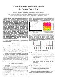
Basic Principle – Diffraction I<br />
• Diffractions are relevant in shadowed areas and are therefore important<br />
• Diffraction loss depending on:<br />
- angle of incidence & angle of diffraction<br />
- properties of material: epsilon, µ and sigma<br />
- polarisation of incident wave<br />
- UTD coefficients with Luebbers extension for modelling the diffraction<br />
Q D<br />
i<br />
k<br />
© by <strong>AWE</strong> <strong>Communications</strong> GmbH 11
<strong>Wave</strong> <strong>Propagation</strong> <strong>Model</strong>s<br />
Basic Principle – Diffraction II<br />
• UTD coefficients with Luebbers extension for modelling the diffraction<br />
• Fresnel function F(x)<br />
• Distance parameter L(r) depending on type of incident wave<br />
© by <strong>AWE</strong> <strong>Communications</strong> GmbH 12
<strong>Wave</strong> <strong>Propagation</strong> <strong>Model</strong>s<br />
Basic Principle – Diffraction III<br />
• Uniform Geometrical Theory of Diffraction (3 zones: NLOS, LOS, LOS + Refl.)<br />
Diffractions are relevant<br />
in shadowed areas<br />
© by <strong>AWE</strong> <strong>Communications</strong> GmbH 13
<strong>Wave</strong> <strong>Propagation</strong> <strong>Model</strong>s<br />
Basic Principle – Knife-Edge Diffraction I<br />
• According to Huygens-Fresnel principle the obstacle acts as secondary source<br />
• Epstein-Petersen: Subsequent evaluation from Tx to Rx (first TQ2 then Q1R)<br />
• Deygout: Main obstacle first, then remaining obstacles on both sides<br />
© by <strong>AWE</strong> <strong>Communications</strong> GmbH 14
<strong>Wave</strong> <strong>Propagation</strong> <strong>Model</strong>s<br />
Basic Principle – Knife-Edge Diffraction II<br />
• Additional diffraction losses in shadowed areas are accumulated<br />
• Determination of obstacles based on Fresnel parameter<br />
• Similar procedure as for Deygout model (start with main obstacle)<br />
• Example:<br />
Height in m<br />
Distance in 50m steps<br />
© by <strong>AWE</strong> <strong>Communications</strong> GmbH 15
<strong>Wave</strong> <strong>Propagation</strong> <strong>Model</strong>s<br />
Basic Principle – Scattering<br />
• Scattering occurs on rough surfaces<br />
• Subdivision of terrain profile into numerous scattering elements<br />
• Consideration of the relevant part only to obtain acceptable computation effort<br />
• Example: Ground properties<br />
Low attenuation if incident angle<br />
equals scattered angle:<br />
Specular reflection<br />
Absorber<br />
Measurement results: RCS with respect to incident<br />
angle alpha and scattered angle beta<br />
(independent of azimuth)<br />
Measurement setup<br />
Ground<br />
© by <strong>AWE</strong> <strong>Communications</strong> GmbH 16
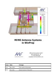
<strong>Wave</strong> <strong>Propagation</strong> <strong>Model</strong>s<br />
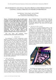
Consideration of Antenna Patterns<br />
• Manufacturer provides 3D antenna pattern<br />
• Manufacturer provides antenna<br />
gains in horizontal and vertical plane<br />
Kathrein K 742212<br />
G <br />
Z<br />
Theta<br />
Bilinear interpolation of 3D antenna characteristic<br />
<br />
<br />
G , <br />
<br />
1 2 1 2<br />
1G2 2G1 1G2 2G1 <br />
<br />
2 2<br />
1 2 1 2<br />
<br />
<br />
1 2 1 2<br />
12 12 <br />
<br />
2 2<br />
1 2 1 2<br />
<br />
G<br />
-Y<br />
<br />
2<br />
1<br />
G <br />
1<br />
2<br />
G <br />
Phi<br />
X<br />
© by <strong>AWE</strong> <strong>Communications</strong> GmbH 17