Computational Approaches to Superconductivity, Research Report ...

Computational Approaches to Superconductivity, Research Report
2006-2012
The main activity of our Minerva Research Group, estabilished in July 2009, is the study of complex solids, in
particular superconductors, using ab-initio DFT calculations. In collaboration with other groups, we combine
these techniques with more traditional many-body methods.
1 Understanding the electronic structure, magnetism and superconductivity
of iron superconductors
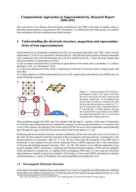
Superconductivity in compounds containing iron (Fe) was considered impossible until 2008, when a critical
temperature (T c ) of 26 K was reported in F-doped LaOFeAs. After this first report, dozens of related compounds
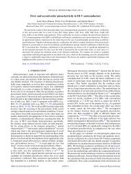
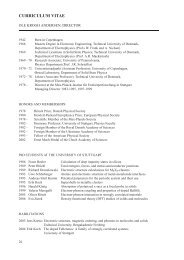
were synthesized, with critical temperatures up to 56 K in SmOFeAs.[2] Fig. 1 shows the basic features that
characterize these Fe superconductors (FeSC):
(a)-(b) A common structural motive, consisting of square planes of iron atoms, andX 4 tetrahedra;X is either a
pnictogen - As,P - or a chalchogen - Se,Te.
(c) A quasi-two-dimensional Fermi surface, comprising two hole and two electron sheets, strongly nested with
each other. 1
(d) A phase diagram, in which superconductivity sets in after suppressing a spin density wave (SDW) state, by
means of doping or pressure.
a)
b)
c)
Γ
Y
M
X
d)
Figure 1: Common features of Fe-based superconductors
(FeSC): FeX layers, seen from
the top (a) and side (b); Fe andX atoms are red
and green, respectively. (c) Two-dimensional
Fermi surface of LaOFeAs, from Ref. [6], with
the hole and electron pockets centered at ¯X, Ȳ
and ¯M respectively. Here a third hole pocket at
¯Γ is also present. (d) Phase diagram, showing
the transition from a spin density wave (SDW)
to a superconducting (SC) state;xis an external
tuning parameter (doping, pressure).
These properties suggest that FeSC may form together with the high-T c cuprates a wide class of compounds,
in which the superconducting pairing is mediated by magnetic excitations (spin fluctuations). In contrast to the
d-wave of the cuprates, the topology of the Fermi surface of FeSC favours in most compounds a superconducting
gap with opposite signs on the hole and electron sheets of the Fermi Surface (s ± ). [4]
Performing and understanding electronic structure calculations, [5] has been the main focus of our activity in
this field. We have studied in detail the formation of the non-magnetic electronic structure, explaining the weak
electron-phonon (ep) interaction - Refs. [6, 7, 8, 9]. We have shown that the description of the SDW state is
problematic in the standard local spin density functional theory (LSDFT) approach, due to the cohexistence
of itinerant and localized magnetic moments - Refs. [6, 10]. This lead us to two different approaches to go
beyond standard LSDFT calculations: combining self-consistent antiferromagnetic (AFM) and non-magnetic
(NM) calculations to estimate the ep coupling in the paramagnetic (PM) state, [11] and using the Gutzwiller
approximation to include strong local correlations. [12] Finally, we have used LSDFT calculations to interpret
experimental data, i.e. optics, [13] phonons [14], spin susceptibilty and specific heat. [15]
1.1 Non-magnetic Electronic Structure
In the region of the phase diagram where superconductivity is observed, Angle Resolved Photoemission (ARPES)
and de-Haas-van-Alphen experiments [16, 17] find the typical Fermi surface topology sketched in Fig. 1(c), with
1 Here and in the following, we do not consider the 122 Fe chalchogenides, [3] which are anomalous in many respects.
1

hole and electron pockets at the center and edges of the Brillouin zone. Theoretical models for superconductivity
mediated by spin-fluctuations (SF) rely on this topology, and on the modifications induced by structural deformation
and three dimensional dispersions, to explain the trends in critical temperatures and gap symmetry in
different FeSC. [18, 19] Non-magnetic DFT calculations reproduce the experimental Fermi surfaces quite well,
except for a moderate to strong quasi-particle renormalization, and a sistematic relative shift of the hole and
electron pockets. [20]
Understanding the formation of this peculiar electronic structure is a highly non-trivial task. [6] We have used
2
xy xy xy
2
xz xz Xz
2
yz yz Yz
2
XY XY XY
1
1
1
1
0
0
0
0
-1
-1
-1
-1
-2
-2
-2
-2
-3
-3
-3
-3
-4
-4
-4
-4
Γ X M Γ
Γ X M Γ
Γ X M Γ
Γ X M Γ
2
z z z
2
x x X
2
y y Y
2
zz zz zz
1
1
1
1
0
0
0
0
-1
-1
-1
-1
-2
-2
-2
-2
-3
-3
-3
-3
-4
-4
-4
-4
Γ X M Γ
Γ X M Γ
Γ X M Γ
Γ X M Γ
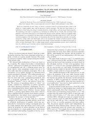
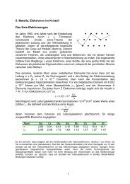
Figure 2: Band structure of the two-dimensional tigh-binding model for a single FeAs layer of
LaOFeAs (2D LaOFeAs). The five Fed(xy,xz,yz,XY =x 2 −y 2 andzz=3z 2 −1) and three
Asp(x,y,z) NMTO’s are shown in the insets. Thexandy axes are directed along the shortest
Fe-Fe distance in Fig. 1 – From Ref. [6].
the NMTO downfolding method [21] to derive an accurate model of the two-dimensional band structure of
LaOFeAs (2D LaOFeAs). Using the symmetry properties of the single FeAs layer, we could exactly reduce the
problem to a single Fe unit cell, and derive an accurate analytical tight-binding model, with five Fe d and three
As p orbitals. Including the As p orbitals explicitely allowed us to study the material trends with tetrahedral
angle [18, 22] and the effect of three-dimensional dispersion, also for those compounds in which As is replaced
by a different ligandX, such as P, Se or Te.
Fig. 2 shows the corresponding bands, decorated with a fatness proportional to the partial character of the orbitals
shows in the small insets. This complicated electronic structure derives from a subtle interplay between the
covalent bonding of Fe t 2 (xz,yz andxy) and Asporbitals, and direct metallic bonding for the Fe e states. The
dashed line marks the position of the Fermi level (E F ) for the nominal electron countp 6 d 6 of most undoped Fe
based superconductors. The Fermi surface is shown in Fig. 1 (c); the states at E F are all oft 2 character, and the
curvature of the bands that form the hole and electron pockets is strongly affected by Fe-As hybridization.
One of the properties of this electronic structure, around the filling p 6 d 6 , is a weak coupling of the electronic
states to phonons – the total electron-phonon coupling constantλ=0.2, is even lower than in elemental aluminum
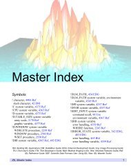
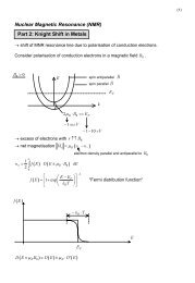
(λ = 0.44), which has a T c of ∼ 1 K, as we have shown in Ref. [7]. The top panel of Fig. 3 shows the
results of a linear-response calculation for LaOFeAs. [23] The phonon spectrum extends up to ∼ 500 cm −1 ,
with a weak ep coupling, distributed among three peaks of Fe-As character at ω 100, 200 and 300 cm −1 . The
distribution of theep spectral functionα 2 F(ω) (Eliashberg function) is uniform, indicating no strong dormantep
interaction. [24, 25]. The lower panel of the same figure shows a similar calculation for the analogous compound,
in which Fe is replaced by nickel - LaONiAs. This compound is also superconducting, but with a much lower
T c 5 K, and the nominal filling is p 6 d 8 . Here, the Fermi level sits ∼ 1 eV higher in Fig. 2, crossing the
states derived from the directed x 2 − y 2 orbitals. Single-band Migdal Eliashberg theory for phonon-mediated
superconductivity is sufficient to explain the experimental T c ’s, and several experimental observations such as
the specific heat jump at T c and the size of the superconducting gap – Refs. [7, 8]. Similar results are found for
other iron and nickel compounds. [26]
2

DOS
α 2 F(ω)
500
400
λ q
ν
La
Fe
As
O
ω (cm -1 )
300
200
100
0
Γ X M Γ Z R A
0 0.2
DOS
0.2
α 2 F(ω)
500
400
λ q
ν
La
Ni
As
O
ω (cm -1 )
300
200
100
0
Γ X M Γ Z R A 0 0.2
0.4 0.8
Figure 3: Phonon dispersion, density of states
(DOS) andep spectral function –α 2 F(ω) – calculated
in density functional perturbation theory
[23] for LaOFeAs (top) and LaONiAs (bottom).
The dashed line represents λ(ω) =
2 ∫ ω
0 α2 F(Ω)dΩ – From Refs. [7, 8].
If E F is shifted further up, until an electron count p 6 d 10−x , the ep matrix elements are even higher, due to the
strong hybridization with the X p states. This is realized in BiOCu 1−x S, where the Cu-S layers play the role
of the Fe-X layers – Ref. [9]. For this material, we have studied the competition of spin fluctuations and ep
coupling, using linear response calculations and the local spin-density functional version of the random-phase
approximation (RPA) for spin fluctuations. We have shown that BiOCu 1−x S is a quite unique compound where
both a conventional phonon-driven and an unconventional triplet superconductivity are possible, and compete
with each other. We argued that, in this case, it may be possible to switch from conventional to unconventional
superconductivity by varying such parameters as doping or pressure.
1.2 The SDW state: problems and hints from DFT calculations
In a large part of their phase diagram – red in Fig. 1 (d) – many FeSC exhibit long-range magnetic order; the most
common pattern is aQ = (0,π) SDW, in which the the Fe spins are aligned aligned ferromagnetically along one
of the edges of the Fe squares, and antiferromagnetically along the other, forming parallel stripes. For this reason,
this pattern is usually called AFM stripe. In this AFM state, the lattice often displays a small orthorhombic
distortion. 11 and 122 chalchogenides exhibit a double-stripe and a block-AFM pattern respectively. Local spin
density functional calculations encounter several problems in describing the formation and suppression of this
magnetic order. In Ref. [10] we have shown for the first time that it is impossible to reproduce, within a single
DFT calculation, the correct value of electronic (fermiology, magnetic moment) and structural (tetrahedral angle,
B 1g phonon frequency) properties. We have interpreted this as an indication that in actual FeSC two types of
magnetic moments cohexist. [30]
The problem is the following: The magnetic moments measured byµSR and inelastic neutron scattering typically
range from 0.5-0.6 – 1.0µ B in the pnictides, to∼2.0µ B for the 11 chalchogenides. The magnetic ground state
in LSDFT is the same SDW order observed by experiments, but the magnitude of the magnetic moment (∼ 2.0
µ B ) is almost independent on the compound, and often much larger than the experimental one. Even worse,
for a large range of dopings for which experiments see no trace of long-range magnetic order, LSDFT equally
predicts an AFM ground state, with m ∼ 2.0 µ B . The puzzling thing is that suppressing this large ordered
moment in the calculations spoils the almost perfect agreement with experiment for the structural and vibrational
properties, introducing errors as large as 25 % for some phonon frequencies, and for the internal position of the
X atoms. [11, 28, 29]
In order to understand the origin and implications of this surprising resut, in Ref. [6] we have studied a simplified
model for AFM in FeSC. This is an extension of the so-called extended Stoner theory for itinerant ferromagnets
[31], which we have recently used to study spin fluctuations in Ni 3 Al, [32] and is usually a very good
approximation to the full self-consistent DFT result. [31, 33] A staggered magnetic field ∆ Q , with the same
3

m/∆(µ B
eV -1 )
2
1.8
1.6
1.4
1.2
1
Q=(0,π)
I=0.59 eV
I=0.82 eV
x=0.00
x=0.05
x=0.10
x=0.15
x=0.20
0 0.5 1 1.5 2 2.5
m(µ B
)
Y
Γ
Y
Γ
M
X
M
X
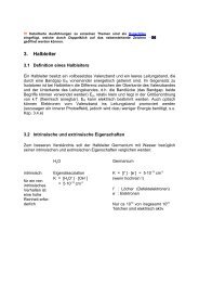
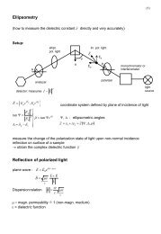
Figure 4: Non-interacting, static spin susceptibilities
χ(m)=m/∆ for 2D LaOFeAs from a
Stoner model for AFM stripes m is the magnetization,
I the Stoner parameter, ∆ the applied
staggered magnetic field, andxis doping in the
rigid band approximation. For a given value
of the Stoner interaction parameter, I, the selfconsistent
moment is given by χ(m) = 1/I.
I = 0.59 and I = 0.82 yield the experimental
and LSDFT value of the magnetic moment,
respectively. The two corresponding Fermi surfaces
are also shown. From Ref. [6].
periodicityQof the SDW, is applied to a system, coupling the k and k+Q blocks of the corresponding tightbinding
Hamiltonian. The resulting magnetizationm is related to∆via the self-consistency condition∆ = mI,
where I is the Stoner interaction parameter, which in LSDFT calculations is set by the choice of the exchange
and correlation functional. Using the 2D tight-binding Hamiltonian for LaOFeAs of Ref. [6] and an orbitalindependent
exchange field for the Fedorbitals, we obtained the non-interacting static spin susceptibilityχ(m)
plotted in Fig. 4, as: χ(m) = m/∆, for several rigid-band dopings x. The curve shown in the figure is for an
AFM stripe – Q = (0,π). This function is uniquely determined by the non-interacting band structure of Fig. 2.
Its shape reflects two different regimes for magnetism: (a) a small moment regime (m ≤ 1.0), dominated by the
strong nesting between hole and electron Fermi pockets, where magnetism is very feeble, and rapidly suppressed
by doping; and a more robust large moment regime (m ≥ 1.0µ B ), which persists up to very high dopings. The
two values ofI represented by dashed lines were chosen to reproduce the ordered moment of LaOFeAs detected
by experiments (m ∼ 0.4µ B ,I = 0.59eV ), [27] and the value found in self-consistent LSDFT calculations (m
∼ 2.0 µ B , I = 0.82 eV). At the side of the figure, we also show the two corresponding Fermi surfaces. These
are qualitatively very different: the small-moment one is reminiscent of the non-magnetic (NM) Fermi surface
shown in Fig. 1 (c), with small SDW gaps; in the large moment one, there is an almost complete reconstruction,
due to a 10 times larger exchange splitting (∆ ∼ 2 eV). ARPES experiments in magnetic samples show Fermi
surfaces similar to the small-moment one; the second topology is never observed. The two Fermi surfaces give a
pictorial representation of the problems encountered by LSDFT in the pnictides: the fermiology and the suppression
of the magnetic moment with doping is well reproduced by small moment calculations, which correspond
to an exchange field of ∼ 2 − 300 meV; in order to reproduce the structural properties, instead, much larger
exchange fields∼ 2 eV are required.
What we proposed in Ref. [10] is that these two regimes cohexist in actual FeSC samples, with large, localized
moments that extend in the whole phase diagram, even the regions where experiments see no trace of static
magnetism. [30] The superconducting samples are thus strongly paramagnetic, i.e. very distant from the nonmagnetic
DFT picture.
1.3 Magnetism, going beyond Density Functional Theory
We proposed a model the paramagnetic state in DFT in Ref. [11], where we studied the effect of magnetism
on phonon dispersions and electron-phonon coupling. The three top panels of fig. 5 show the results of
three self-consistent calculations of phonon dispersions and ep coupling for BaFe 2 As 2 , with a ground state
which is non-magnetic (NM), anti-ferromagnetic with a checkerboard pattern (AFMc), and anti-ferromagnetic
stripe (AFMs). The thick, colored lines represent the phonon densities of states (DOS), the dashed lines give
the same-spin component of the Eliashberg function: α 2 F σσ (ω). The corresponding ep coupling constants
λ σσ = 2 ∫ dωα 2 F σσ (ω)/ω are 0.18, 0.33 and 0.18 respectively. The average ep matrix elements of the two
AFM calculations (λ σσ /N σ (0)=0.25) are about 1.5 time larger than the NM result (λ/N(0)=0.15), due to magnetoelastic
coupling. We obtained an estimate of the coupling in the paramagnetic phase, combining the phonon
frequencies andep matrix elements of the AFM solution, with the Fermi surface given by the non-magnetic calculati
ons. The resultingep spectal functionα 2 F(ω) is plotted in blue in Fig. 5 together with the non-magnetic
one; the increased weight around 20 meV yields a 50 % increase in the total ep coupling. The corresponding
phonons are the B 1g Raman-active modes that distort the tetrahedra. From this result, together with a rigid-band
approximation for doping, we estimated a new upper bound for the ep coupling in the paramagnetic phase of
FeSC, λ PM = 0.35. This value, which is twice as large as the one estimated in the NM phase [7], is still too
4

F(ω)
0.2
0.1
0
0.2
0.1
0
0.2
0.1
NM
λ=0.18
N σ
(0)=1.18
AFMc
λ=0.33
N σ
(0)=1.36
AFMs
λ=0.18
N σ (0)=0.68
tot
Fe
As
0
0 10 ω (meV) 20 30
10 ω (meV) 20 30
0.3
α 2 F(ω)
0.2 λ(ω)
0.1
PM
NM
Figure 5: Top panel: Phonon DOS (full lines)
and same-spin ep spectral function α 2 F σσ(ω)
(dashed line) for non-magnetic (NM), antiferromagnetic
checkerboard (AFMc) and
antiferromagnetic stripe (AFMs) BaFe 2As 2.
Lower panel: α 2 F σσ(ω) and λ σσ(ω) for
non-magnetic (NM) and paramagnetic (PM)
BaFe 2As 2. – From Ref. [11].
m/µ B
2.5
2.0
1.5
1.0
0.5
J=0.10U
J=0.075U
J=0.05U
Stoner
0.0
0.4 0.5 0.6 0.7 0.8 0.9
I/eV, χDFT −1 /eV
Figure 6: Ordered stripe magnetic moment
m of undoped, 2D LaOFeAs as a function of
I eff = U −0.017J, in the Gutzwiller approximation
(red, green, blue symbols), together
with the inverse of the non-interacting spin susceptibility
χ −1 (m), shown in fig. 4. – From
Ref. [12].
low to explain the superconducting T c alone, but is high enough to yield visible effects in realistic models for
the pairing.
The cohexistence of localized and itinerant moments in FeSC can only be captured by methods that include local
fluctuations, such as the dynamical mean field theory (DMFT). The solution of multiband Hubbard models, in
which the kinetic part is given by realistic models of the DFT band structure (LDA+DMFT), reproduces a state
with small ordered moments and large local fluctuating moments. [34] A very similar picture is given by the
simpler Gutzwiller approximation. [35]. In Ref. [12], we solved a multiband Hubbard Hamiltonian, in which
the kinetic part is given by the 8-band model of Ref. [6], and the full atomic interaction between the electrons
in the iron orbitals is parametrized by the Hubbard interactionU and an average Hund’s-rule interaction J. We
found that for a wide range of (U,J) parameters the ground state is a metallic spin density wave (SDW), with
a small magnetic moment. The local moment (< S 2 >∼ 2.0µ B ) is much larger than the ordered one, but still
far from the fully polarized atomic value (m = 4.0µ B ). Consistently with the DMFT results, we found that the
value of the magnetic moment is mostly determined by the Hund’s coupling J. Indeed, Fig. 6 shows that the
results for different sets of calculations collapse onto a single curve, if the moment is plotted as a function of the
effective Stoner parameterI = J −0.017U. For comparison, the inverse of the static susceptibility at x = 0 is
also shown; the good agreement between the two curves indicates that the magnetically ordered phase is a stripe
spin-density wave of quasiparticles.
1.4 Interpretation of experimental spectra
In Ref. [13] we compared model calculations of the intraband optical spectra, treated in a multi-band Eliashberg
model, experimental data [36] and first-principles calculations, to show that interband transitions give a non
negligible contribution already in the infrared region of the spectrum. This leads to a substantial failure of the
extended-Drude-model analysis on the measured optical data without subtraction of interband contributions.
5

As a consequence the electron-boson coupling gets dramatically overestimated. This effect was also recently
measured by the Keimer Department. [37]
In Ref. [14], in collaboration with the group of Bernhard Keimer, we have analyzed the anomalous dependence
of the c-axis B 1g phonon in FeSe/Te samples, using Raman scattering and first-principles calculations.
The local density calculations, including magnetic polarization and Fe nonstoichiometry in the virtual crystal
approximation, reproduce well the experimental data in the Fe-deficient samples, while the effects of Fe excess
are poorly reproduced. This may be due to excess Fe-induced local magnetism and low-energy magnetic
fluctuations that cannot be treated accurately within these approaches. In Ref. [15], we have investigated the
specific heat and upper critical fields of KFe 2 As 2 . The measured Sommerfeld coefficient γ n =94(3) mJ/mol K 2
of KFe 2 As 2 is anomalously large, but this is due to extrinsic effects. Taking this into account, KFe 2 As 2 should
be classified as a weakly or intermediately coupled superconductor with a total electron-boson coupling constant
λ tot =1 (including a calculated weak electron-phonon couplingλ ph =0.17).
2 Superconductivity in intercalated picene
Studying carbon, with its many allotropes and compounds, is one of the most fascinating problems in science.
To mention only physics, before graphene, which was awarded the Nobel prize in 2010 for opening exciting perspectives
for fundamental and applied research, many other systems such as nanotubes, fullerenes, intercalated
graphites have played an important role in several fields, including superconductivity.
5
0 1 2 3 800 4 1600 2400 6 3200
ω (cm -1 )
1 2 3
4 5 6
Figure 7: Top: Structure of a picene
molecule, and of the corresponding crystal.
Bottom: Phonon spectrum of crystalline picene
in DFPT [23], showing representative vibration
patterns. The modes 4 and 5, in red, give the
highest contribution to ep coupling in our rigid
band calculations. – From Ref. [45].
The most recent discovery is a new class of aromatic superconductors, comprising molecular crystals doped
with alkali or alkaline earths metals. These are polycyclic aromatic hydrocarbons, i.e. planar molecules formed
by a number of juxtaposed hexagonal benzene rings (C 6 H 6 ). The first report of superconductivity in this class of
materials concerned picene doped with potassium (K) and rubidium (Rb) with a maximum critical temperature
(T c ) of 18 K [38]. After that, superconductivity was also found in phenanthrene and coronene doped with K
(T c =5K and 15 K), [39, 40] phenanthrene doped with strontium (Sr) and barium (Ba) (T c =5.6-5.8 K) [41], and
1,2:8,9-dibenzopentacene(C 30 H 18 ) doped with K (T c =33 K) [42]. Intercalated hydrocarbons are strongly related
to two families of carbon superconductors: graphite intercalation compounds (GICs), which are conventional,
BCS-like superconductors [43] and alkali-doped fullerenes (A 3 C 60 ), which instead have a rich phase diagram
determined by a non-trivial interplay between strong localep interactions and on-site Coulomb correlations in a
highly non-adiabatic regime [44].
In Ref. [45] we performed first-principles calculations of the electronic structure, phonon spectra and electronphonon
(ep) interaction of doped picene in the rigid band approximation (RBA), using density functional perturbation
theory (DFPT). Based on our results for the vibrational properties, and on previous studies on electronic
properties and correlations, we showed that picene, and most likely other intercalated hydrocarbons, belong to
a class of strongly correlatedep superconductors, for which a local approach that includes both the ep coupling
6

and Coulomb correlations on an equal footing may be more appropriate. The main results of our study are summarized
in Fig. 7. The top panel shows the structure of the isolated picene molecules, and their arrangement in
a crystal; the lower panel shows the spectrum of crystalline picene calculated in LDA; in the inset, typical displacements
are shown. The modes indicated in red are those which give a larger contribution to theep coupling.
The molecularep matrix element, isV ep = 150±20 meV for holes andV ep = 110±5 meV for electrons. These
values are comparable to the bandwidth of the conduction band (W∼300 meV) and typical phonon frequencies
(ω ph ∼ 200 meV).
For a rigid-band doping of picene with ∼ 3 electrons per molecule, N(E F ) = 7.06 states spin −1 meV −1 , λ =
0.78 andω ln = 1021 cm −1 . Usingµ ∗ = 0.12 in the McMillan formula, we obtain a critical temperatureT c = 56.5
K. This is more than three times the experimental value of T c , and we need to use a larger value of µ ∗ = 0.23
to reproduce the experimental T c . However, it is important to stress that the estimates of T c based on Migdal-
Eliashberg theory must be taken with care in the case of picene. In fact, the bandwidth of the conduction bands
(W ∼ 300 meV for electrons and ∼ 1 eV for holes), the frequencies of strongly coupled phonons (ω ph ∼ 200
meV), theep coupling strength (V ep ∼ 110-150 eV), all have similar magnitudes, close also to that of Coulomb
repulsion (U ∼ 1.2 eV), estimated by other authors [46]. In this range of parameters, the two most important
approximations in Migdal-Eliashberg theory of superconductivity, Migdal’s theorem and the Morel-Anderson
scheme for the screening of the Coulomb repulsion, are invalid. In fullerenes, this regime of parameters gives
rise to a variety of interesting phenomena, the most spectacular being the occurrence of ep superconductivity
near a Mott insulating phase, well captured by theoretical studies of local models of interacting phonons and
electrons in the non-adiabatic regime. [44]
This first study motivated us to start a collaboration on electronic and vibrational properties of intercalated
hydrocarbons, with the high-pressure and optics group of Università la Sapienza, in Rome. [47]
3 Iridates
Recently, Ohgushi et al. reported resonant x-ray diffraction study of CaIrO 3 that indicates this material exhibits
a Mott insulating J eff = 1/2 state [48]. Previously, it was found that spin-orbit coupling can play an important
role in the electronic properties even for a 4d 5 system such as Sr 2 RhO 4 [49, 50]. Since CaIrO 3 is a 5d 5 system,
this material provides a more oppurtune platform to study the interplay between spin-orbit coupling and onsite
Coulomb repulsion. Furthermore, this material proffers a playground for a recent theory that suggests
that systems in the J eff = 1/2 state, depending on bond geometry, lead to interesting varieties of low-energy
Hamiltonians [51]. The density functional calculations within the local density approximation showed that the
spin-orbit coupling splits the Ir t 2g bands into fully filled quartet of J eff = 3/2 bands and half-filled doublet of
J eff = 1/2 bands [52]. This metallic state is contrary to the experiments that show that CaIrO 3 is an insulator.
However, the half-filled J eff = 1/2 bands have a band width of ∼1 eV and a value for the on-site Coulomb
repulsion ofU = 2.75 eV yields a Mott insulating state. The LDA+SO+U calculations give an antiferromagnetic
ground state for CaIrO 3 along the c axis with total moments aligning antiparallel along the c axis, in agreement
with the experiment. For U = 2.75 eV, the total magnetic moment is 0.67 µ B , with an orbital contribution of
0.28 µ B and a spin contribution of 0.38 µ B . These values differ from what is expected for the ideal J eff = 1/2
state, and this deviation might be explained by the mixing of J eff =1/2 bands with Ir e g bands due to the tilting
of IrO 6 octahedra.
Note: Our Minerva Research Group was estabilished in July 2009; before this, L. Boeri was a staff member in
the Andersen Department (Electronic Structure Theory). For consistency, all the activity on fe-based superconductors
is reported here.
References
[1] Y. Kamihara, T. Watanabe, M. Hirano, and H. Hosono, J. Am. Chem. Soc. 130, 3296 (2008).
[2] J. Paglione and R. L. Greene, Nature Phys. 6, 645 (2010); D. C. Johnston, Adv. Phys. 59, 803 (2010);
special issue of Rep. Prog. Phys. , vol. 74, 2011.
[3] J. Guo, S. Jin, G. Wang, S. Wang, K Zhu, T. Zhou, M. He, and X. Chen, Phys. Rev. B 82, 180520 (2010).
[4] P. J. Hirschfeld, M. M. Korshunov, I. I. Mazin, Rep. Prog. Phys. 74, 124508 (2011).
7

[5] to mention only a few early works: S. Lebegue, Phys. Rev. B 75 035110 (2007); D. J. Singh and M.-H. Du,
Phys. Rev. Lett. 100, 237003 (2008); D. J. Singh, Phys. Rev. B 78, 094511 (2008); Alaska Subedi, Lijun
Zhang, D. J. Singh, and M. H. Du, Phys. Rev. B 78, 134514 (2008); Alaska Subedi, Lijun Zhang, D. J.
Singh, and M. H. Du, Phys. Rev. B 78, 134514 (2008); I. I. Mazin, D. J. Singh, M. D. Johannes, and M.
H. Du, Phys. Rev. Lett. 101, 057003 (2008). K. Kuroki, Seiichiro Onari, Ryotaro Arita, Hidetomo Usui,
Yukio Tanaka, Hiroshi Kontani, and Hideo Aoki, Phys. Rev. Lett. 101, 087004 (2008), Verónica Vildosola,
Leonid Pourovskii, Ryotaro Arita, Silke Biermann, and Antoine Georges, Phys. Rev. B 78, 064518 (2008),
for the basic electronic structure; For magnetism: T. Yildirim, Phys. Rev. Lett. 101, 057010 (2008); S.
Ishibashi, K. Terakura, and H. Hosono, J. Phys. Soc. Jpn. 77 (2008) 053709; Z. P. Yin,et al, Phys. Rev.
Lett. 101, 047001 (2008).
[6] O. K. Andersen and L. Boeri, Ann. Phys. (Leipzig) 523, 8 (2011).
[7] L. Boeri, O. V. Dolgov, and A. A. Golubov, Phys. Rev. Lett. 101, 026403 (2008).
[8] L. Boeri, O. V. Dolgov, and A. A. Golubov, Physica C 469, 628 (2009).
[9] L. Ortenzi, S. Biermann, O. K. Andersen, I. I. Mazin, and L. Boeri, Phys. Rev. B 83, 100505(R) (2011).
[10] I. I. Mazin, M. D. Johannes, L. Boeri, K. Koepernik, and D. J. Singh, Phys. Rev. B 78, 085104 (2008).
[11] L. Boeri, M. Calandra, I. I. Mazin, O. V. Dolgov, and F. Mauri, Phys. Rev. B 82, 020506 (2010).
[12] T. Schickling, F. Gebhard, J. Bünemann, L. Boeri, O. K. Andersen, and W. Weber, Phys. Rev. Lett. 108,
036406 (2012).
[13] L. Benfatto, E. Cappelluti, L. Ortenzi, and L. Boeri, Phys. Rev. B 83, 224514 (2011).
[14] Y. J. Um, A. Subedi, P. Toulemonde, A. Y. Ganin, L. Boeri, M. Rahlenbeck, Y. Liu, C. T. Lin, S. J. E.
Carlsson, A. Sulpice, M. J. Rosseinsky, B. Keimer, and M. Le Tacon, Phys. Rev. B 85, 064519 (2012).
[15] M. Abdel-Hafiez, S. Aswartham, S. Wurmehl, V. Grinenko, C. Hess, S.-L. Drechsler, S. Johnston, A. U. B.
Wolter, B. BÃijchner, H. Rosner, and L. Boeri, Phys. Rev. B 85, 134533 (2012).
[16] P Richard, T Sato, K Nakayama, T Takahashi and H Ding, Rep. Prog. Phys. 74, 12451 (2011).
[17] A Carrington, Rep. Prog. Phys. 74, 124507 (2011).
[18] Kazuhiko Kuroki, Hidetomo Usui, Seiichiro Onari, Ryotaro Arita, and Hideo Aoki Phys. Rev. B 79, 224511
(2009).
[19] S. Graser et al., New J. Phys. 11, 025016 (2009); Ronny Thomale, Christian Platt, Werner Hanke, and B.
Andrei Bernevig, Phys. Rev. Lett. 106, 187003 (2011), and many others.
[20] L. Ortenzi, E. Cappelluti, L. Benfatto, and L. Pietronero, Phys. Rev. Lett. 103, 046404 (2009).
[21] O. K. Andersen and T. Saha-Dasgupta, Phys. Rev. B 62, R16219 (2000).
[22] C.-H. Lee, A. Iyo, H. Eisaki, H. Kito, M.T. Fernandez-Diaz, T. Ito, K. Kihou, H. Matsuhata, M. Braden,
and K. Yamada, J. Phys. Soc. Jpn. 77, 083704 (2008).
[23] Stefano Baroni, Stefano de Gironcoli, Andrea Dal Corso, and Paolo Giannozzi, Rev. Mod. Phys. 73, 515
(2001).
[24] W. Weber, L. F. Mattheis, Phys. Rev. B 25, 2248 and 2270 (1982).
[25] L. Boeri, J. Kortus, and O. K. Andersen, Phys. Rev. Lett. 93, 237002 (2004).
[26] Alaska Subedi and David J. Singh, Phys. Rev. B 78, 132511 (2008); Alaska Subedi, Lijun Zhang, D. J.
Singh, and M. H. Du, ibid 134514; Alaska Subedi, David J. Singh, and Mao-Hua Du, ibid 060506 (2008).
[27] C. de la Cruz, et al., Nature (London) 453, 899 (2008); (poly) m=0.36µ B ; more recent reports yield larger
values of the magnetic moment. See: N. Qureshi et al. ,Phys. Rev. B 82, 184521 (2010). (polycrystals)
m=0.63µ B ; H.F. Li et al., Phys. Rev. B 82, 064409 (2010) m=0.8µ B (single + poly-crystals).
[28] M. Zbiri, et al, Phys. Rev. B 79, 064511 (2009);
[29] D. Reznik, et al, Phys. Rev. B 80, 214534 (2009).
8

[30] I. I. Mazin and M. D. Johannes, Nature Physics 5, 141 - 145 (2009).
[31] O.K. Andersen, J. Madsen, U.K. Poulsen, O. Jepsen, and J. Kollár Physica B&C 86-88, 249 (1977).
[32] L. Ortenzi, L. Boeri, P. Blaha and I.I. Mazin, submitted.
[33] O. Gunnarsson, J. Phys. F: Metal Phys. 6, 587 (1976).
[34] M. Aichhorn et al., Phys. Rev. B 80, 085101 (2009) and ibid., 054529 (2011); P. Hansmann et al., Phys.
Rev. Lett. 104, 197002 (2010); Z.P. Yin, K. Haule, and G. Kotliar, Nature Phys. 7, 294 (2011).
[35] M. C. Gutzwiller, Phys. Rev. 137, A1726 (1965).
[36] M.M. Qazilbash, J.J. Hamlin, R.E. Baumbach, L. Zhang, D.J. Singh, M.B. Maple, and D.N. Basov, Nature
Physics 5, 647 (2009).
[37] A. Charnukha, P. Popovich, Y. Matiks, D.L. Sun, C.T. Lin, A.N. Yaresko, B. Keimer, and A. V. Boris, Nat.
Comm. 2, 219 (2011).
[38] R. Mitsuhashi, Y. Suzuki, Y. Yamanari, H. Mitamura. T. Kambe, N. Ikeda, H. Okamoto, A. Fujiwara, M.
Yamaji, N. Kawasaki, Y. Maniwa, and Y. Kubozono, Nature (London) 464, 76 (2010).
[39] X. F. Wang, R. H. Liu, Z. Gui, Y. L. Xie, Y. J. Yan, J. J. Ying, X. G. Luo, and X.H. Chen, Nat. Commun. 2,
507 (2011).
[40] Y. Kubozono, H. Mitamura, X. Lee, X. He, Y. Yamanari, Y. Takahashi, Y. Suzuki, Y. Kaji, R. Eguchi, K.
Akaike, T. Kambe, H. Okamoto, A. Fujiwara, T. Kato, T. Kosugi and H. Aoki, Phys. Chem. Chem. Phys.
13, 16476 (2011).
[41] X. F. Wang, Y. J. Yan, Z. Gui, R. H. Liu, J. J. Ying, X. G. Luo, and X. H. Chen, Phys. Rev. B 84, 214523
(2011).
[42] M. Xue, T. Cao, D. Wang, Y. Wu, H. Yang, X. Dong, J. He, F. Li, G. F. Chen, arXiv:1111.0820.
[43] T. E. Weller et al., Nature Phys. 1, 39 (2005); N. Emery et al., Phys. Rev. Lett. 95, 087003 (2005); J. S.
Kim et al., Phys. Rev. Lett. 99, 027001 (2007).
[44] A. F. Hebard et al., Nature 350, 600 (1991); O. Gunnarsson, Alkali-Doped Fullerides (World Scientific,
Singapore 2004); A. Y. Ganin et al., Nature Mater. 7, 367 (2008); M. Capone et al., Rev. Mod. Phys. 81,
943 (2009).
[45] A. Subedi and L. Boeri, Phys. Rev. B 84, 020508(R) (2011).
[46] G. Giovannetti and M. Capone, Phys. Rev. B 83, 134508 (2011).
[47] B. Joseph, L. Boeri et al., Journal of Physics Cond. Matter (2012).
[48] K. Ohgushi, J.-I. Yamaura, H. Ohsumi, K. Sugimoto, S. Takeshita, A. Tokuda, H. Takagi, M. Takata, and
T.-H. Arima, e-print arXiv:1108.4523.
[49] M. W. Haverkort, I. S. Elfimov, L. H. Tjeng, G. A. Sawatzky, and A. Damascelli, Phys. Rev. Lett. 101,
026406 (2008).
[50] G.-Q. Liu, V. N. Antonov, O. Jepsen, and O. K. Andersen, Phys. Rev. Lett. 101, 026408 (2008).
[51] G. Jackeli and G. Khaliullin, Phys. Rev. Lett. 102, 017205 (2009).
[52] A. Subedi, Phys. Rev. B 85, 020408(R) (2012).
9