Diploma thesis - Fachbereich Physik

More documents

Recommendations

Info

40 CHAPTER 3. RECURSION RELATIONS 3.2 Ground-State Energy without External Current For the potential the time-independent Schrödinger equation reads − ¯h2 2M ψ′′ (x) + V (x) = M 2 ω2 x 2 + gAx 3 + g 2 Bx 4 , (3.4) ( M 2 ω2 x 2 + gAx 3 + g 2 Bx 4 ) ψ(x) = E ψ(x) . (3.5) Inserting the ansatz (3.2) into the Schrödinger equation (3.5) yields an ordinary differential equation for the correction φ(x): − ¯h2 2M φ′′ (x) + ¯hω x φ ′ (x) − ¯h2 2M [φ′ (x)] 2 + gAx 3 + g 2 Bx 4 = ǫ , (3.6) where ǫ denotes the correction to the ground-state energy E = ¯hω 2 + ǫ . (3.7) Expanding the ground-state energy of the oscillator in powers of the coupling constant g, E = ¯hω ∞ 2 + ∑ g k ǫ k , (3.8) k=1 inserting the expansion (3.3) into (3.6), and performing a coefficients comparison, one obtains a differential equation for the φ k (x): − ¯h2 2M φ′′ k (x) + ¯hω x ¯h2 φ′ k (x) − 2M ∑k−1 φ ′ k−l (x) φ′ l (x) + δ k,1Ax 3 + δ k,2 Bx 4 = ǫ k . (3.9) l=1 Assuming that φ k (x) is a polynomial, one can show by induction that its degree cannot be greater than k + 2. Thus, the φ k (x) can be written in the form ∑k+2 φ k (x) = m=1 c (k) m xm . (3.10) Here, the constant terms c (k) 0 have been omitted as they can only be determined later by normalization of the wave function ψ(x). By inserting (3.10) into (3.9) for k = 1, one finds c (1) 1 = − A Mω 2 , For k = 2, the solution reads c (2) 1 = 0 , c (2) 2 = 7A2 8M 2 ω − 3B 4 4Mω , 2 c(1) 2 = 0 , c (1) 3 = − A 3¯hω , and ǫ 1 = 0 . (3.11) c(2) 3 = 0 , c (2) 4 = A2 8M¯hω − B 3 4¯hω , (3.12) and ǫ 2 = − 11A2¯h 2 8M 3 ω 4 + 3B¯h2 4M 2 ω 2 . (3.13)
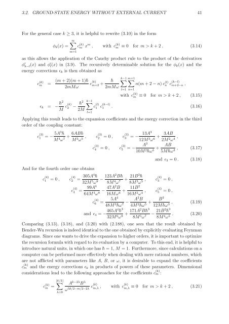
3.2. GROUND-STATE ENERGY WITHOUT EXTERNAL CURRENT 41 For the general case k ≥ 3, it is helpful to rewrite (3.10) in the form ∞∑ φ k (x) = c (k) m xm , with c (k) m ≡ 0 for m > k + 2 , (3.14) m=1 as this allows the application of the Cauchy product rule to the product of the derivatives φ ′ k−l (x) and φ′ l (x) in (3.9). The recursively determinable solution for the φ k(x) and the energy corrections ǫ k is then obtained as c (k) m ǫ k = (m + 2)(m + 1)¯h 2mMω = −¯h2 M c(k) 2 − ¯h2 2M c (k) ¯h m+2 + 2mMω ∑k−1 l=1 ∑ ∑ k−1 m+1 l=1 n=1 with c (k) m n(m + 2 − n) c (l) n c (k−l) m+2−n , ≡ 0 for m > k + 2 , (3.15) c (l) 1 c(k−l) 1 . (3.16) Applying this result leads to the expansion coefficients and the energy correction in the third order of the coupling constant: c (3) 1 = − 5A3¯h M 4 ω 7 + 6AB¯h M 3 ω 5 , And for the fourth order one obtains c(3) 2 = 0 , c (3) 3 = − 13A3 12M 3 ω 6 + 3AB 2M 2 ω 4 , c (3) 4 = 0 , c (3) 5 = − A3 10M 2¯hω 5 + c (4) 1 = 0 , c (4) 2 = 305A4¯h 32M 5 ω − 123A2 B¯h + 21B2¯h 9 8M 4 ω 7 8M 3 ω , 5 c (4) 4 = 99A4 64M 4 ω 8 − 47A2 B 16Mω 6 + 11B2 16M 2 ω 4 , c (4) 6 = 5A 4 48M 3¯hω 7 − AB 5M¯hω 3 , (3.17) and ǫ 3 = 0 . (3.18) c(4) 3 = 0 , c(4) 5 = 0 , A2 B 4M 2¯hω 5 + B 2 12M¯hω 3 , (3.19) and ǫ 4 = − 465A4¯h 3 32M 6 ω 9 + 171A2 B¯h 3 8M 5 ω 7 − 21B2¯h 3 8M 4 ω 5 . (3.20) Comparing (3.13), (3.18), and (3.20) with (2.188), one sees that the result obtained by Bender-Wu recursion is indeed identical to the one obtained by explicitly evaluating Feynman diagrams. Since one wants to drive the expansion to higher orders, it is important to optimize the recursion formula with regard to its evaluation by a computer. To this end, it is helpful to introduce natural units, in which one has ¯h = 1, M = 1. Furthermore, since calculations on a computer can be performed more effectively when dealing with mere rational numbers, which are not afflicted with parameters like A, B, or ω, it is desirable to expand the coefficients and the energy corrections ǫ k in products of powers of these parameters. Dimensional considerations lead to the following approaches for the coefficients c (k) c (k) m m : ⌊k/2⌋ c (k) m = ∑ A k−2λ B λ c(k) ω5k/2−m/2−2λ m,λ , λ=0 with c(k) m,λ ≡ 0 for m > k + 2 , (3.21)
Page 1: Beyond Effective Potential via Vari
Page 4 and 5: 4 CONTENTS 4.5 Potential with Cubic
Page 6 and 7: 6 CHAPTER 1. INTRODUCTION ries. For
Page 9 and 10: Chapter 2 Effective Action In addit
Page 11 and 12: 2.2. DEFINITION OF THE EFFECTIVE AC
Page 13 and 14: 2.3. DEFINITION OF THE EFFECTIVE PO
Page 15 and 16: 2.4. EXAMPLE: HARMONIC OSCILLATOR 1
Page 17 and 18: 2.4. EXAMPLE: HARMONIC OSCILLATOR 1
Page 19 and 20: 2.5. EXAMPLE: ORDINARY INTEGRAL 19
Page 21 and 22: 2.6. BACKGROUND METHOD: ORDINARY IN
Page 23 and 24: 2.7. BACKGROUND METHOD: PATH INTEGR
Page 29 and 30: 2.8. CALCULATION OF THE EFFECTIVE P
Page 31 and 32: 2.9. EXAMPLE: ANHARMONIC OSCILLATOR
Page 33 and 34: 2.9. EXAMPLE: ANHARMONIC OSCILLATOR
Page 35 and 36: 2.10. PERTURBATION THEORY 35 the fo
Page 37: 2.10. PERTURBATION THEORY 37 To obt
Page 42 and 43: 42 CHAPTER 3. RECURSION RELATIONS a
Page 44 and 45: 44 CHAPTER 3. RECURSION RELATIONS U
Page 46 and 47: 46 CHAPTER 3. RECURSION RELATIONS k
Page 48 and 49: 48 CHAPTER 3. RECURSION RELATIONS l
Page 51 and 52: Chapter 4 Variational Perturbation
Page 53 and 54: 4.2. ARBITRARY COUPLING STRENGTH 53
Page 55 and 56: 4.4. POTENTIAL WITH QUARTIC ANHARMO
Page 57 and 58: 4.4. POTENTIAL WITH QUARTIC ANHARMO
Page 59 and 60: 4.5. POTENTIAL WITH CUBIC ANHARMONI
Page 67 and 68: Chapter 5 Extension to D Dimensions
Page 69 and 70: 5.1. OSCILLATOR WITH QUARTIC ANHARM
Page 75 and 76: 5.2. BACKGROUND METHOD FOR EFFECTIV
Page 85: 5.2. BACKGROUND METHOD FOR EFFECTIV
Page 88 and 89: 88 CHAPTER 6. OUTLOOK where the ima
Page 91 and 92:
Appendix A Harmonic Generating Func
Page 93 and 94:
93 Evaluating the x 0 -, Re x m -,
Page 95:
95 and that the eigenvalues of G
Page 98 and 99:
98 APPENDIX B. STANDARD INTEGRALS R
Page 100 and 101:
100 APPENDIX B. STANDARD INTEGRALS
Page 103 and 104:
Appendix C Shooting Method In this
Page 105:
x → −∞, or vice-versa. Thus,
Page 109:
List of Figures 4.1 Schematic compa
Page 113 and 114:
Bibliography [1] Physik Journal 3 (
Page 115:
BIBLIOGRAPHY 115 [29] W. Janke and
show all

Diploma thesis - Fachbereich Physik

You also want an ePaper? Increase the reach of your titles

Delete template?

Save as template?