Diploma thesis - Fachbereich Physik

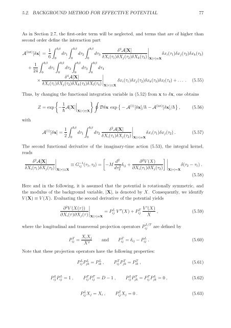
5.2. BACKGROUND METHOD FOR EFFECTIVE POTENTIAL 77
As in Section 2.7, the first-order term will be neglected, and terms that are of higher than
second order define the interaction part
A (int) [δx] = 1 ∫ ¯hβ ∫ ¯hβ ∫ ¯hβ
δ 3 A[X]
dτ 1 dτ 2 dτ 3
6 0 0 0 δX i (τ 1 )δX j (τ 2 )δX k (τ 3 ) ∣ δx i (τ 1 )δx j (τ 2 )δx k (τ 3 )
X(τ)≡X
+ 1 ∫ ¯hβ ∫ ¯hβ ∫ ¯hβ ∫ ¯hβ
dτ 1 dτ 2 dτ 3 dτ 4
24 0 0 0 0
δ 4 A[X]
×
δX i (τ 1 )δX j (τ 2 )δX k (τ 3 )δX l (τ 4 ) ∣ δx i (τ 1 )δx j (τ 2 )δx k (τ 3 )δx l (τ 4 ) + . . . . (5.55)
X(τ)≡X
Thus, by changing the functional integration variable in (5.52) from x to δx, one obtains
Z = exp
{− 1¯h ∣ } ∮
A[X]
∣∣X(τ)≡X
Dδx exp { − A (1) [δx]/¯h − A (int) [δx]/¯h } , (5.56)
with
A (1) [δx] = 1 2
∫ ¯hβ
0
∫ ¯hβ
dτ 1 dτ 2
0
δ 2 A[X]
δX i (τ 1 )δX j (τ 2 ) ∣ δx i (τ 1 )δx j (τ 2 ) . (5.57)
X(τ)≡X
The second functional derivative of the imaginary-time action (5.53), the integral kernel,
reads
]∣
δ 2 A[X]
δX i (τ 1 )δX j (τ 2 ) ∣ ≡ G −1
ij (τ 1, τ 2 ) =
[−M d2 ∂ 2 V (X) ∣∣∣X(τ)=X
δ ij +
δ(τ 2 − τ 1 ) .
X(τ)≡X
∂X i (τ 1 )∂X j (τ 2 )
dτ 2 2
(5.58)
Here and in the following, it is assumed that the potential is rotationally symmetric, and
the modulus of the background variable, |X|, is denoted by X. Consequently, we identify
V (X) ≡ V (X). Evaluating the second derivative of the potential yields
∂ 2 V (X(τ))
∂X i (τ)∂X j (τ) ∣ = Pij L V ′′ (X) + Pij
T
X(τ)≡X
V ′ (X)
X , (5.59)
where the longitudinal and transversal projection operators P L/T
ij
are defined by
P T
ij = X iX j
X 2 and P T
ij = δ ij − P L
ij . (5.60)
Note that these projection operators have the following properties:
P L
ijP L jk = P L
ik ,
P T
ijP T jk = P T
ik , (5.61)
P L
ij P L
ij = 1 ,
P T
ij P T
ij = D − 1 ,
P L
ij P T jk = P T
ij P L jk = 0 , (5.62)
P L
ij X j = X i ,
P T
ij X j = 0 . (5.63)