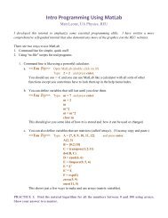
MatLab Programming – Lesson 2

MatLab Programming – Lesson 2
1) Log into your computer and open MatLab…
2) If you don’t have the previous M-scripts saved, you can find them at
http://www.physics.arizona.edu/~physreu/dox/matlab_lesson_1.pdf.
Review 2-D Graphing
Copy the following script into a new M-file.
close all; clear all; clc; format short;
% Its not usually smart to condense lines like above
% (hard to read later), but with the beginning stuff I
% usually do anyway.
x = linspace(0,3,1000);
y_a = x;
y_b = x.^2;
y_c = sin(x);
y_d = exp(x);
y_e = log(x);
plot(x,y_a,x,y_b,x,y_c,x,y_d,x,y_e); % Multiple plots on single graph.
legend('linear','quadratic1','sinusoidal',...
'exponential','logarithmic',2);
% Triple dots allows you to wrap lines (so you can see better).
% Use the help menu to find out what the '2' does for ‘legend’
(search ‘legend’ in the help index).
Now replace the plot command with:
plot(x,y_a,'go', x,y_b,'b.',...
x,y_c,'r-', x,y_d,'k:',...
x,y_e,'p--',...
'markersize',10,'markerfacecolor','y');
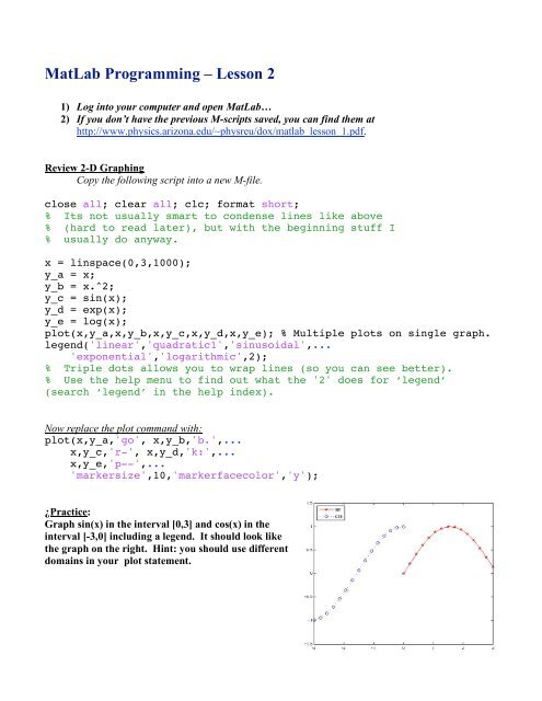
¿Practice:
Graph sin(x) in the interval [0,3] and cos(x) in the
interval [-3,0] including a legend. It should look like
the graph on the right. Hint: you should use different
domains in your plot statement.

More 3-D Graphing
A contour plot shows the height of a function. Copy the following script into a new M-file.
close all;clear all;clc;format short;
x = linspace(-2, 2, 30);
y = linspace(-2, 2, 30);
[X,Y] = meshgrid(x,y);
z = (X-1).^2 + Y.^2;
% This is the function of a depression located
% at x=1 and y=0.
contour(X,Y,z,25);
% The 25 colored contour lines show the height
% of z.
xlabel('x'); ylabel('y');
¿Practice:
Use a contour plot to find the min and max of sin(x)*sin(y) in the interval -10 < x < 10, and
-10 < y < 10.

More 3-D Graphing
A surfc plot is in 3-D and shows the contours. Copy the following script into a new M-file.
close all;clear all;clc;format short;
x = linspace(-5, 5, 100);
y = linspace(-5, 5, 100);
[X,Y] = meshgrid(x,y);
z = sin(X).*sin(Y);
surfc(X,Y,z);
colormap copper;
% Colormaps allow you to process the
% color of images to your own specifications.
xlabel('x'); ylabel('y'); zlabel('z');
¿Practice:
Find a cool function for z to make a surfc plot. Dress up the plot with some fancy commands.
Perhaps it will be a picture for your web site!

More 3-D Graphing
‘plot3’ simply graphs x-y-z coordinates (not as useful as you would think). Copy the following
script into a new M-file.
close all;clear all;clc;format short;
x = linspace(1,10*pi,1000);
plot3(sin(x),cos(x),x);
% Plot a 3-D spiral.
grid on;
xlabel('x'); ylabel('y'); zlabel('z');

While Loops
A while loop continues until a condition is met. Copy the following script into a new M-file.
close all; clear all; clc; format short;
x = 0;
n_count = 0;
while x < 99,
x = 100*rand(1);
n_count = n_count + 1;
end;
if abs(n_count - 300) < 1e-9,
break;
end;
% Always include an escape for a while loop
% in case you screw up the programming. Otherwise,
% you might get caught in an infinite loop.
if n_count < 300,
disp(['It took ',num2str(n_count),' random tries to beat 99.']);
% Re-run this program several times. What is the largest
% n_count you found? Compare with a neighbor.
else,
disp('Timed out!');
end;
¿Practice:
Write a program that creates takes the natural logarithm of a random number between 1 and 100
until it is larger than 4.6 using a while loop. What is the smallest number of times your random
number has to be generated in any single run of your program?

Exporting Data (SKIP THIS SECTION FOR NOW, GO TO LESSON 3.)
You can create a file to store data by opening, printing and closing. Copy the following script into
a new M-file.
close all; clear all; clc; format short;
outfile = fopen('my_data.txt','wt');
x = 0;
n_count = 0;
while x < 99,
x = 100*rand(1);
n_count = n_count + 1;
fprintf(outfile,'%10d %+6.3f\n',n_count,x);
end;
if abs(n_count - 300) < 1e-9,
break;
end;
% Always include an escape for a while loop
% in case you screw up the programming. Otherwise,
% you might get caught in an infinite loop.
if n_count < 300,
disp(['It took ',num2str(n_count),' random tries to beat 99.']);
% Re-run this program several times. What is the largest
% n_count you found? Compare with a neighbor.
else,
disp('Timed out!');
end;
fclose(outfile);
¿Practice:
Write a program that randomly generates the ages of 100 people between the values of 0 and 110.
Do not give all ages equal weight, but let older ages be less likely. Hint: try taking one minus the
negative exponential of a random number and multiplying the result by 110,
110*(1-exp(-rand(1,100))). Export this to a .txt data file.

Importing Data (SKIP THIS SECTION FOR NOW, GO TO LESSON 3.)
You can open a data file using load. Copy the following script into a new M-file.
close all; clear all; clc; format short;
load my_data.txt;
% Creates array called 'my_data' with
% stored values as elements (super handy).
n_size = size(my_data,1);
% Find out how many rows of data there are.
n_sum = 0;
for i_loop = 1:n_size,
end;
if my_data(i_loop,2) > 50,
n_sum = n_sum + 1;
end;
% This loop counts how many times the random number
% was above 50.
disp([num2str(n_sum),' random number were above 50.']);
¿Practice:
Write a program that reads into memory the data file of random birthdays that you created in the
previous section. Have you program count the number of birthdays above 50. Does the weighting
algorithm you used to generate the data seem realistic?
Note: It took me days to figure out a more complicated importing of data. If you have a giant data set
that is much too large to load into your memory all at once, you can read it in line by line. See my
program http://bohr.physics.arizona.edu/~leone/pj/p_visualize.pdf.

Inline Functions (SKIP THIS SECTION FOR NOW, GO TO LESSON 3.)
Sure MatLab knows sin, cos, exp, and several other functions. But you can create your own
functions inside your program to be called later. Later you will learn how to call functions that are entire
separate programs. Copy the following script into a new M-file.
close all;clear all;clc;format short;
% Let's make some variables to use in our functions:
a = 5;
b = 3.5;
% NOW MAKE SOME FUNCTIONS.
myfunction = inline('x + y','x','y');
% Make a function that uses two input variables.
% NOW USE THE FUNCTIONS.
myfunction(a,b)
% Leave ';' off so it prints to screen and you can see it.
¿Practice:
Make a program that asks the user for a radius, uses an inline function to calculate the area, and
then displays the area.

Inline Functions (more) (SKIP THIS SECTION FOR NOW, GO TO LESSON 3.)
Inline functions can be used with scalar data (just single numbers) or with arrays or numbers. Be
sure your inline function uses ‘dotted functions’ where appropriate to operate on arrays element-byelement.
Copy the following script into a new M-file.
close all; clear all; clc; format short;
% Let's make some variables to use in our functions:
a = 5;
b = 3.5;
c = pi^pi;
G = 10*rand(20,3);
D = rand(20,3);
D(:,1) = 2*D(:,1)-1;
D(:,2) = 3*D(:,2);
D(:,3) = 4*D(:,3);
% D(:,1) means take all rows and the first column. It
% is the same as typing D(1:end,1).
% NOW MAKE SOME FUNCTIONS.
f_triggy = inline('(sin(x)*(cos(x)))/log(y)','x','y');
% Make a function that uses two input variables.
f_power = inline('(x.^y)./z','x','y','z');
% Make a weird power function that uses three variables
% that could possibly be arrays with the same dimensions.
% NOW USE THE FUNCTIONS.
% 1) Try f_triggy with numbers.
fprintf('1\n');
f_triggy(a,b)
% Leave ';' off so it prints to screen and you can see it.
fprintf('\n\n\n')
% 2) Try f_power with numbers.
fprintf('2\n');
f_power(a,b,c)
fprintf('\n\n\n')
% 3) Try f_triggy with numbers.
fprintf('3\n');
f_triggy(G,D)
% This function was not set up to multiply arrays
% element-by-element; go back and fix it.
fprintf('\n\n\n')
% 4) Try f_power with numbers.

fprintf('4\n');
f_power(G,D,D) % This function works.
fprintf('\n\n\n')
¿Practice:
a) Make your program have a function that is able to take matrix inputs and perform some math
operations with them element-by-element.
b) Now write a program that creates a data set matrix of real numbers with a size of 10000 X 4
where each element is between -100 and 100 in size. Here is a partial example:
M =
-98.1582 19.4765 -68.8456 3.9074
13.8492 39.9856 72.0272 -57.8941
19.7625 -31.5866 -83.6175 22.5648
7.5571 -36.8443 -93.9813 -30.9987
-76.5710 -34.4167 -20.5149 79.9511
-36.2071 -18.6431 2.2775 -72.2470
-0.0191 -61.5494 32.8980 1.1866
-69.4575 56.4274 -30.9396 -40.2943
35.6457 -1.9173 -18.6166 -92.8042
-47.9353 -16.0275 -93.9745 50.6888
… and so on…
c) Have your program save this data as a text file. Now save this data file to your website and
include a link to it on your web page.
d) Create another program that reads in a data file and adds all the numbers inside together with
the command sum(sum(M)). Go to another participants web site and download their data, then run
your program on their data.
(END OF LESSON 2)