Technical University Kaiserslautern Preprint - Fachbereich Physik ...

Parametric Resonance in Bose-Einstein Condensates
William Cairncross ∗
Institut für Theoretische Physik, Freie Universität Berlin, Arnimallee 14, D-14195 Berlin, Germany and
Department of Physics, Queen’s University at Kingston, Canada
Axel Pelster †
Fachbereich Physik und Forschungszentrum OPTIMAS,
Technische Universität Kaiserslautern, Germany and
Hanse-Wissenschaftskolleg, Lehmkuhlenbusch 4, D-27733 Delmenhorst, Germany
(Dated: September 13, 2012)
We demonstrate parametric resonance in Bose-Einstein condensates (BECs) with attractive twobody
interaction in a harmonic trap under parametric excitation by periodic modulation of the
s-wave scattering length. We obtain nonlinear equations of motion for the widths of the condensate
using a Gaussian variational ansatz for the Gross-Pitaevskii condensate wave function. We conduct
both linear and nonlinear stability analyses for the equations of motion and find qualitative agreement,
thus concluding that the stability of two equilibrium widths of a BEC might be inverted by
parametric excitation.
PACS numbers: 67.85.Hj,03.75.Kk
The phenomenon of parametric resonance, when a system
is parametrically excited and oscillates at one of its
resonant frequencies, is ubiquitous in physics: the phenomenon
is found from simple classical systems such as
the child’s swing and the vertically driven pendulum [1],
tothePauliontrap[2]andaspectsofsomeinflationmodels
of the universe [3]. Parametrically excited systems
are usually nonlinear: even the parametrically driven
pendulum is governed by the linear Mathieu equation
onlyfor smalloscillationsabout its equilibrium positions.
Nonetheless, valuable qualitative insight into these systems
may be gained by investigating their behavior in
the vicinity of equilibrium points.
In the realm of ultracold quantum gases, initial studies
of parametric resonance have featured Faraday patterns
[4–6], Kelvin waves of quantized vortex lines [7],
self-trapped condensates [8, 9], bright and vortex solitons
[10, 11], and self-damping at zero temperature [12].
Recently, it was shown for a shaken optical lattice that a
periodic driving can even induce a quantum phase transition
from a Mott insulator to a superfluid [13, 14],
paving the way for new techniques to engineer exotic
phases [15, 16]. Other novel experimental techniques
[17, 18] to excite a Bose-Einstein condensate (BEC) of
7 Li in the vicinity of a broad Feshbach resonance [19] by
harmonic modulation of the s-wave scattering length, in
contrastto the usual method of excitation by modulation
of the trapping potential [20–23], have inspired investigations
of parametric resonance and other phenomena
in Refs. [11, 25–27]. Conspicuously absent from these
investigations is a study of the simplest case of parametric
resonance in Bose-Einstein condensates: a systematic
stability analysis for the parametrically excited
three-dimensional BEC in a harmonic trap. Therefore,
we conduct in this letter a lucid proof-of-concept study
of such a parametrically excited BEC by demonstrating
that within both a linear analytic and a nonlinear numeric
analysis the stability characteristics of its equilibrium
configurations can be changed.
We start with modeling the dynamics of a BEC at zero
temperature using the mean-field Gross-Pitaevskii (GP)
Lagrangian
∫ [ i
L(t) =
(ψ ∂ψ∗ −ψ ∗∂ψ
)− 2
2 ∂t ∂t 2m |∇ψ|2
]
−V(r)|ψ| 2 − 2π2 a(t)
m |ψ|4 dr. (1)
The functional derivative of the Lagrangian results in
the well-known GP equation for the dynamics of the
mean-field condensate wave function ψ = ψ(r,t). In experimentsgenericallyacylindrically-symmetricharmonic
trapping potential V(r) = mω 2 ρ (ρ2 + λ 2 z 2 )/2 is used,
whose elongation is described by the trap anisotropy parameter
λ = ω z /ω ρ . Furthermore, we assume that the s-
wave scattering length is periodically modulated according
to
a(t) = a 0 +a 1 sinΩt. (2)
In the following we will investigate how the stability of
condensate equilibria depends on both the driving amplitude
a 1 and the driving frequency Ω, provided the
time-averageds-wave scattering length a 0 is slightly negative.
In principle, this could be analyzed by solving the
underlying GP equation for the condensate wave function
ψ = ψ(r,t), which follows from extremizing the Lagrangian
(1). However, the thorough numerical analysis
in Ref. [25] demonstrated convincingly that the dynamicsofthe
GPequationcanbe well-approximatedwithin a
Gaussian variational ansatz for the GP condensate wave
function [28, 29]. Even for long evolution times and in

2
the vicinity of resonances, where oscillations of the condensate
are quite large, it was possible to reduce the GP
partial differential equation to a set of ordinary differential
equations for the variational parameters.
Therefore, we follow the latter approach and employ
the Gaussian ansatz
]
ψ G (ρ,z,t) = N(t)exp
[− ρ2
+iρ 2 φ ρ
2ũ 2 ρ
]
×exp
[− z2
2ũ 2 +iz 2 φ z , (3)
z
with time-dependent variational widths ũ ρ , ũ z , phases
φ ρ , φ z , andnormalizationN(t) = N 1/2 π 3/2 ũ −1
ρ ũ−1/2 z .Inserting
the Gaussian ansatz (3) into the GP Lagrangian
(1) and extremizing with respect to all variational parameters,
we obtain at first explicit expressions for the
phases φ ρ,z = m˙ũ ρ,z /(2ũ ρ,z ). We define the dimensionless
time τ = ω ρ t and scale the variational widths
by u ρ,z = ũ ρ,z /a ho , where a ho = √ /(mω ρ ) is the harmonic
oscillator length. Finally, we write the dimensionless
driving function p(τ) = p 0 +p 1 sin(Ωτ/ω ρ ) according
to the definitions p 0,1 = √ 2/πNa 0,1 /a ho . The resulting
dynamics for the widths u ρ and u z is then determined
by a pair of coupled nonlinear ordinary differential equations:
ü ρ +u ρ = 1 u 3 ρ
ü z +λ 2 u z = 1 u 3 z
+ p(τ)
u 3 ρu z
,
+ p(τ)
u 2 ρu 2 . (4)
z
For attractive two-body interactions, there exists a
critical value of the time-averaged interaction strength
p crit
0 (λ) < 0 beyond which no equilibria exist in the absence
of parametric driving. Its dependence on the trap
anisotropy λ must be evaluated numerically, as for example
in Ref. [27]. For p crit
0 (λ) < p 0 < 0, there exists a
pair ofequilibrium points for Eqs. (4), one stable and one
unstable [28, 29], which we denote with u 0+ and u 0− , respectively.
Weremarkthatthe stabilityofthesepointsin
the absence of parametric driving is determined by evaluating
the frequencies of collective modes for small oscillations
about equilibrium [27]. Whereas the equilibrium
u 0+ hasrealfrequenciesforallmodesand, thus, is stable,
the equilibrium u 0− possessesanimaginaryfrequencyfor
one mode, implying exponential behaviour and thus instability.
In view of a linear stability analysis we assume small
oscillations about an equilibrium, write u ρ ≈ u ρ0 + δu ρ
and u z ≈ u z0 + δu ρ , and expand the nonlinear terms
of Eqs. (4) to first order in δu ρ and δu z . We scale and
translate time as 2t ′ +π/2 = Ωτ/ω ρ , define displacement
and forcing vectors x(t ′ ) and f,
( ) ⎛
p
δuρ (τ) (
x(t ′ ωρ
)
1
⎞
2 u
) = , f = 4 ⎝
3 ρ0 uz0
⎠, (5)
δu z (τ) Ω
p 1
u 2 ρ0 u2 z0
and finally we introduce the matrices A and Q corresponding
to constant and periodic coefficients, respectively:
A = 4
Q = −2
⎛
( ωρ
) 2
⎝
Ω
⎛
( ωρ
) 2
⎝
Ω
4
2p 0
u 3 ρ0 u2 z0
p 0
u 3 ρ0 u2 z0
3λ 2 + 1
u 4 z0
3
u 4 ρ0 uz0 1
u 3 ρ0 u2 z0
2
u 3 ρ0 u2 z0
2
u 2 ρ0 u3 z0
⎞
⎞
⎠,
⎠. (6)
The result is a set of coupled, asymmetric, inhomogeneous
Mathieu equations,
ẍ(t ′ )+(A−2p 1 Qcos2t ′ )x(t ′ ) = f cos2t ′ , (7)
whose solutions determine whether the underlying equilibrium
is stable or unstable.
The Mathieu equation, a special case of Hill’s differential
equation [30], has been studied extensively in the
literature [31]: approaches to obtaining the equation’s
stability diagram include continued fractions [30, 32, 33],
perturbative methods [34–36], and infinite determinant
methods [37–40]. The problem has been treated in great
detail in Ref. [41] for the study of the Paul trap, the stability
of which is governed exactly by a set of coupled
homogeneous Mathieu equations. Of importance to our
particular problem are Refs. [42, 43], where it was shown
that for both single and coupled Mathieu equations, an
inhomogeneous term does not affect the location of stability
borders to Eq. (7). In the following, we choose the
concisecontinued-fractionmethod basedontheapproach
of Refs. [32, 33].
The π-periodic parametric driving of the Mathieu
equation permits the application of Floquet theory, the
essential statement of which is that each of the two fundamental
solutions x 1,2 (t ′ ) to Eq. (7) may be written in
the form [44]
x 1,2 (t ′ ) = e ±βt′
∞ ∑
n=−∞
b 2n e 2int′ , (8)
where the π-periodic part consists of Fourier components
b 2n and the exponential part is characterized by the Floquet
exponent β, which determines the stability of the
solution. Due to the presence of both signs of the exponent
in a general solution, we require for stability that
R[β] = 0. On the stability borders, solutions to the
Mathieu equation are mπ-periodic with m ∈ Z. Thus to
obtain the stability borders, we set β = mi in Eq. (8).
By substitution of the Floquet ansatz(8) into Eq. (7), we
obtain a third-order recurrence relation for the Fourier
coefficients b 2n :
[ ]
A+(β +2in) 2 I b 2n −p 1 Q(b 2n+2 +b 2n−2 ) = 0. (9)

3
We define the ladder operators S ± 2n b 2n = b 2n±2 as
S ± 2n = {A+[β +2i(n+1)] 2 I−p 1 QS ± 2n±2} −1p1
Q,
(10)
and by repeated re-substitution of these ladder operators
into the recursion relation (9) for n increasing and
decreasing from zero, we obtain a tri-diagonal matrixvalued
continued fraction relating the parameters A, Q,
and β:
( { [ ] −1
A+β 2 I−p 2 1 Q A+(β +2i) 2 −...
[ ] } ) −1
+ A+(β −2i) 2 −... Q b 0 = 0. (11)
In order to obtain a non-trivial solution for b 0 , the
determinant of the matrix-valued continued fraction in
Eq. (11) must vanish. The resulting stability for a particular
value of the modulation frequency Ω and the dimensionless
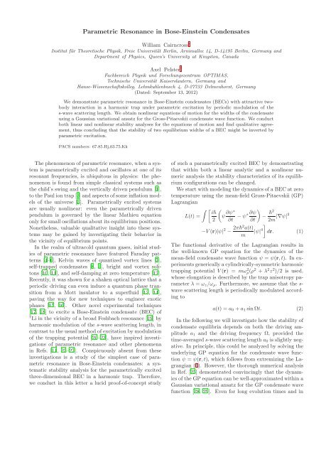
driving amplitude p 1 is then shown in the
linear stability diagram of Fig. 1 for three characteristic
values of the trap anisotropy λ. Our results indicate that
for the unstable (stable) equilibrium position, the largest
regionofstability (instability) occursforapancakeBEC,
i.e., for λ > 1.
As a special case the stability borders for the isotropic
condensate are given by a separate continued fraction,
obtained by an analogous process for a single inhomogeneous
Mathieu equation. The resulting stability diagrams
are shown in Fig. 2. It allows to draw a direct
analogy between the isotropic condensate and the parametrically
driven pendulum: the pendulum too is described
by a single Mathieu equation, however the inhomogeneous
term in the equation of motion for the BEC
corresponds to a direct periodic driving in phase with
the parametric driving. It was shown in Ref. [42] that
a periodic inhomogeneity has no effect on the stability
borders for a single Mathieu equation, so Fig. 2 is simply
a transformation of the standard Ince-Strutt stability diagram
for the parametrically driven pendulum [30], for
the relevant experimental parameters of the BEC.
Whiletheresultsoflinearstabilityanalysisforthecoupled
Mathieu system are qualitatively similar to those
for the single equation, there are a number of notable
changes between Figs. 1 and 2. First, for the coupled
Mathieu equations, there exist a set of stability regions
not attainable by the analytic method used here. These
are displayed without black borders in Fig. 1, and correspond
to the so-called “combined resonances” of the system
[39, 41]. These regions are attainable by numerical
stability analysis of the Mathieu equations [41, 44, 45],
which was used to generate the colored background regions
of Fig. 1. It is notable in Fig. 1 that these anomalous
regions are not present for λ = 1.
A second and important difference from the single to
the coupled Mathieu equations is the appearance of a
(a)
(b)
(c)
FIG. 1. Linear stability diagrams for the unstable (case 1)
and stable (case 2) equilibrium positions of a cylindricallysymmetric
BEC for three values of the trap anisotropy λ: (a)
λ = 0.2 (a cigar-shaped BEC), (b) λ = 1 (spherical BEC),
and (c) λ = 2.6 (pancake-shaped BEC). White regions correspond
to unstable solutions, darkest shaded regions to stable
solutions, and lightly shadedregions correspond tomarginally
stable solutions – regions where only one of two available collective
oscillation modes is stable.
new region, shaded white and issuing from Ω/ω ρ ≈ 10 in
Fig. 1 for λ = 1, case 1. This region is identified with the
instability of the quadrupole collective mode, which does
not appear in a one-dimensional analysis. This result
implies that a three-dimensional analysis might result in
further changes to the linear stability diagram of Fig. 1
for λ = 1, case 1.
As the underlying equations of motion (4) are inherently
nonlinear, a linear analytic stability analysis alone
is not sufficient to investigate the phenomenon of parametric
resonance. Therefore, we have also performed a
detailed numerical stability analysis by integrating the
equations of motion (4) over a long time-period using a
Runge-Kutta-Verner 8(9) order algorithm, incrementing
through pairs (p 1 ,Ω) and recording divergent solutions
to obtain the corresponding stability diagram. The corresponding
results are shown in Fig. 3 for the same three
values of the trap anisotropy λ as in Fig. 1.

4
(a)
FIG. 2. Linear stability diagrams for (a) unstable and (b)
stable equilibria of an isotropic BEC. Shaded and white regions
indicate stable and unstable solutions, respectively. The
presence of a stable region in (a) indicates that an originally
unstable equilibrium might be stabilized by parametric excitation.
(b)
The results for the originally stable equilibrium u 0+
show both qualitative and even quantitative similarity
to the linear stability analysis of Fig. 1, i.e., a similar
tonguelike structure of unstable regions issuing from certain
points on the vertical axis. The originally unstable
equilibrium u 0− also shows qualitative similarity to the
linear analysis of Fig. 1, however the region of stability
begins only for much larger modulation frequency Ω
and dimensionless driving amplitude p 1 . These results
are both reasonable, as the linear stability analysis is
only valid for small oscillations – corresponding to large
(p 1 ,Ω) for equilibrium u 0+ and small (p 1 ,Ω) for equilibrium
u 0− . Furthermore, in contrast to Fig. 1, we find
in the nonlinear stability diagram of Fig. 3 that stability
is more easily achieved for a cigar-shaped BEC, i.e., for
λ < 1.
Further comparison of the linear and nonlinear stability
diagrams of Figs. 1 and 3 shows the possibility of
both simultaneous stability of the equilibrium positions,
and even the possibility of a complete reversal of the
stability characteristics. In the latter case, the smaller
equilibrium position would become the only stable width
of the condensate, which should be experimentally observable.
A final observation, applicable to the originally
unstable equilibrium in both linear and nonlinear
cases, is the existence of a minimum driving amplitude
p min
1 necessary to stabilize the condensate. The value
p min
1 = u 0 (5u 4 0−1) ≈ 0.17 p 0 is exactly attainable for the
linearanalysisoftheisotropiccondensate, andinFig.1is
approximately independent of λ in the considered range
[0.2,2.6]. For the nonlinear analysis, p min
1 ≈ 1.2 p 0 is also
approximately independent of λ. This feature will have
implications for an experiment, as in conjunction with
the width of the Feshbach resonance, it dictates the minimum
modulation of the applied magnetic field necessary
to stabilize the condensate.
(c)
FIG. 3. Nonlinear stability diagrams for the unstable (left)
andstable(right)equilibriaofacylindrically-symmetricBEC,
for three values of the trap anisotropy λ: (a) λ = 0.2 (a cigarshaped
BEC), (b) λ = 1 (spherical BEC), and (c) λ = 2.6
(pancake BEC).
Wenotethatanystabilitydiagramdependsontheparticular
choice for the time-averaged dimensionless interaction
strength p 0 . The concrete resultsin Figs. 1–3were
obtained for the particular value p 0 = 0.9 p crit
0 (λ). As p 0
approaches p crit
0 (λ), we generically observe a growth of
the stable (unstable) regions in case 1 (2).
Finally, we conclude that our proof-of-concept investigation
has unambiguously shown that the phenomenon
ofparametricresonanceshouldbeexperimentallyobservable
also for Bose-Einstein condensation. However, due
to the intrinsic nonlinear nature of the underlying GP
mean-field theory, a linear analysis, like in the Paul trap,
is not sufficient to quantitatively study the stability diagram.
Thus, in order to achieve a destabilization (stabilization)
of a stable (unstable) BEC equilibrium in an
experiment, a corresponding numerical nonlinear analysisisindispensable.
Regardless,alinearstability analysis
providesanintuitiveandqualitativeunderstandingofthe
physics of parametric resonance in BECs.
In the present letter we have focused our attention
upon a periodic modulation of the s-wave scattering
length around a slightly negative value, which restricts

5
the number of particles in a BEC to the order of a few
thousand [46, 47]. However, the phenomenon of parametric
resonance might be more important for dipolar
BECs, where in addition to a repulsive short-range and
isotropic interaction, also a long-range and anisotropic
dipolar interaction between atomic magnetic or molecular
dipoles is present. Provided that the dipolar interaction
is smaller than the contact interaction, a stable
dipolar BEC does exist. But a larger dipolar strength
leads to mutual existence of both a stable and an unstabledipolarBEC[48]whosestabilitymightbechangedvia
a periodic modulation of the harmonic trap frequencies
or the s-wave scattering length. In that context it might
also be of interest to estimate how quantum fluctuations,
which are non-negligible for a larger dipolar interaction
strength [49], change the stability diagram. The case
for dipolar Fermi gases is probably even more interesting
from the point of view of parametric resonance, as for
any dipolar strength a stable equilibrium coexists with
an unstable one [50]. Thus, parametric resonance may
offer a simple efficient approach for realizing equilibria of
dipolar quantum gases whose properties have so far not
yet been explored.
We are grateful to Jochen Brüggemann for discussions
and Antun Balažfor his valuable input. This project was
supported by the DAAD (German Academic Exchange
Service) within the program RISE (Research Internships
in Science and Engineering).
∗ william.cairncross@queensu.ca
† http://www.physik.fu-berlin.de/~pelster
[1] R.P. Feynman, R.B. Leighton, and M. Sands, The Feynman
Lectures on Physics, Vol. 1 (Addison-Wesley, New
York, 1964).
[2] W. Paul, Angew. Chem. Int. Ed. Engl. 29, 739 (1990).
[3] L. Kofman, A. Linde and A.A. Starobinsky, Phys. Rev.
Lett. 73, 3195 (1994).
[4] K. Staliunas, S. Longhi, and G.J. de Valcárcel, Phys.
Rev. Lett. 89, 210406 (2002).
[5] P. Capuzzi, M. Gattobigio, and P. Vignolo, Phys. Rev.
A 83, 013603 (2011).
[6] A. Balaz and A.I. Nicolin, Phys. Rev. A 85, 023613
(2012).
[7] T.P. Simula, T. Mizushima, and K. Machida, Phys. Rev.
Lett. 101, 020402 (2008).
[8] H. Saito, R.G. Hulet, and M. Ueda, Phys. Rev. A 76,
053619 (2007).
[9] F.Kh. Abdullaev, J.G. Caputo, R.A. Kraenkel, and B.A.
Malomed, Phys. Rev. A 67, 013605 (2003).
[10] H. Saito and M. Ueda, Phys. Rev. Lett. 90, 040403
(2003).
[11] S.K. Adhikari, Phys. Rev. A 69, 063613 (2004).
[12] Y. Kagan and L.A. Maksimov, Phys. Rev. A 64, 053610
(2001).
[13] A. Eckardt, C. Weiss, and M. Holthaus, Phys. Rev. Lett.
95, 260404 (2005).
[14] A. Zenesini, H. Lignier, D. Ciampini, O. Morsch, and E.
Arimondo, Phys. Rev. Lett. 102, 100403 (2009).
[15] J. Struck, C. Olschlager, R. Le Targat, P. Soltan-Panahi,
A. Eckardt, M. Lewenstein, P. Windpassinger, and K.
Sengstock, Science 333, 996 (2011).
[16] J. Struck, C. Olschlager, M. Weinberg, P. Hauke, J. Simonet,
A. Eckardt, M. Lewenstein, K. Sengstock, and P.
Windpassinger, Phys. Rev. Lett. 108, 225304 (2012).
[17] E. R. F. Ramos and E. A. L. Henn and J. A. Seman
and M. A. Caracanhas and K. M. F. Magalhães and
K. Helmerson and V. I. Yukalov and V. S. Bagnato,
Phys. Rev. A 78, 063412 (2008).
[18] S.E. Pollack, D. Dries, R.G. Hulet, K.M.F. Magalhães,
E.A.L. Henn, E.R.F. Ramos, M.A. Caracanhas, and V.S.
Bagnato, Phys. Rev. A 81, 053627 (2010).
[19] S.E. Pollack, D. Dries, M. Junker, Y.P. Chen, T.A. Corcovilos,
and R.G. Hulet, Phys. Rev. Lett. 102, 090402
(2009).
[20] D.S. Jin, J.R. Ensher, M.R. Matthews, C.E. Wieman,
and E.A. Cornell, Phys. Rev. Lett. 77, 420 (1996).
[21] M.-O. Mewes, M.R. Andrews, N.J. van Druten, D.M.
Kurn, D.S. Durfee, and W. Ketterle, Phys. Rev. Lett.
77, 416 (1996).
[22] D.S. Jin, M.R. Matthews, J.R. Ensher, C.E. Wieman,
and E.A. Cornell, Phys. Rev. Lett. 78, 764 (1997).
[23] J. J. García-Ripoll, V. M. Pérez-García, and P. Torres,
Phys. Rev. Lett. 83, 1715 (1999).
[24] P.G. Kevrekidis, G. Theocharis, D.J. Frantzeskakis, and
B.A. Malomed, Phys. Rev. Lett. 90, 230401 (2003).
[25] I. Vidanovic, A. Balaz, H. Al-Jibbouri, and A. Pelster,
Phys. Rev. A 84, 013618 (2011).
[26] A. Rapp, X. Deng, and L. Santos arXiv:1207.0641
[27] H. Al-Jibbouri, I. Vidanovic, A. Balaz, and A. Pelster,
arXiv:1208.0991.
[28] V.M. Pérez-García, H. Michinel, J.I. Cirac, M. Lewenstein,
and P. Zoller, Phys. Rev. Lett. 77, 5320 (1996).
[29] V.M. Pérez-García, H. Michinel, J.I. Cirac, M. Lewenstein,
and P. Zoller, Phys. Rev. A 56, 1424 (1997).
[30] M. Abramowitz and I. A. Stegun, Handbook of Mathematical
Functions with Formulas, Graphs and Mathematical
Tables (Dover, New York, 1972).
[31] N. W. McLachlan, Theory and Applications of Mathieu
Functions (Oxford, Clarendon, 1947).
[32] H. Risken, The Fokker-Planck Equation (Springer,
Berlin, 1989).
[33] C. Simmendinger, A. Wunderlin, and A. Pelster, Phys.
Rev. E 59, 5344 (1999).
[34] A.H. Nayfeh, Perturbation Methods (Wiley-VCH, Weinheim,
2004).
[35] D. Younesian, E. Esmailzadeh, and R. Sedaghati, Commun.
Nonlinear Sci. Numer. Simul. 12, 58 (2007).
[36] G.M. Mahmoud, Physica A 242, 239 (1997).
[37] K.G. Lindh, Am. Inst. Aer. Astr. J. 8, 680 (1970).
[38] P. Pedersen, Ingenieur-Archiv 49, 15 (1980).
[39] J. Hansen, Ingenieur-Archiv 55, 463 (1985).
[40] H. Landa, M. Drewsen, B. Reznik, and A. Retzker,
arXiv:1206.0716.
[41] A. Ozakin and F. Shaikh, arXiv:1109.2160.
[42] G. Kotowski, Z. Angew. Math. Mech. 23, 213 (1943).
[43] J. Slane and S. Tragesser, Nonlin. Dyn. Syst. Th. 11, 183
(2011).
[44] V.A. Yakubovich and V.M. Starzhinski, Linear differential
equations with periodic coefficients (Wiley, NewYork,
1975).

6
[45] A.A. Mailybaev, O.N. Kirillov, and A.P. Seyranian, J. of
Phys. A: Math. 38, 1723 (2005).
[46] C.C. Bradley, C.A. Sackett, J.J. Tollett, and R.G. Hulet,
Phys. Rev. Lett. 75, 1687 (1995).
[47] C.C. Bradley, C.A. Sackett, J.J. Tollett, and R.G. Hulet,
Phys. Rev. Lett. 79, 1170 (1997).
[48] D.H.J.O’Dell, S.Giovanazzi, andC.Eberlein, Phys.Rev.
Lett. 92, 250401 (2004).
[49] A.R.P. Lima and A. Pelster, Phys. Rev. A 84, 041604(R)
(2011).
[50] T. Miyakawa, T. Sogo, and H. Pu, Phys. Rev. A 77,
061603(R) (2008).