CalEnviroscreen Version 1.1 - OEHHA - State of California

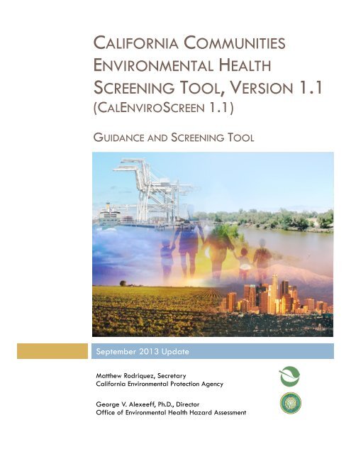
CALIFORNIA COMMUNITIES 

ENVIRONMENTAL HEALTH 

SCREENING TOOL, VERSION 1.1 

(CALENVIROSCREEN 1.1) 

GUIDANCE AND SCREENING TOOL 

September 2013 Update 

Matthew Rodriquez, Secretary 

California Environmental Protection Agency 

George V. Alexeeff, Ph.D., Director 

Office of Environmental Health Hazard Assessment

CalEnviroScreen 1.1 

OEHHA Authors: 

John Faust 

Laura Meehan August 

George Alexeeff 

Komal Bangia 

Rose Cendak 

Lara Cushing 

Tamara Kadir 

Carmen Milanes 

Karen Randles 

Robbie Welling 

Walker Wieland 

Lauren Zeise 

OEHHA Editors: 

Allan Hirsch 

Shankar Prasad 

Cal/EPA Reviewers: 

Miriam Barcellona Ingenito 

Julian Leichty 

Arsenio Mataka 

Gina Solomon 

Acknowledgements: 

Cumulative Impacts and Precautionary Approaches Work Group 

Cal/EPA Boards and Departments who provided comments and data; 

California Department of Public Health and the Public Health Institute 

Residents and stakeholders who participated in our regional workshops; Tara Zagofsky, 

consultant and facilitator, University of California, Davis, Common Ground: Center for 

Cooperative Solutions 

Dr. Rachel Morello-Frosch and academic colleagues at the University of California, Berkeley 

Academic expert panel who provided comments at a workshop in September 2012 

Graduate students assisting in the project, including Christopher Carosino, Laurel Plummer and 

Jocelyn Claude


PREFACE TO VERSION 1.1 

CalEnviroscreen 1.1 is the latest iteration of the CalEnviroScreen tool. It uses the same methodology as 

Version 1.0 except that the indicator for race/ethnicity was removed from the calculation of a 

community’s CalEnviroScreen score. This change was made to facilitate the use of the tool by 

government entities that may be restricted from considering race/ethnicity when making certain decisions. 

While race and ethnicity will not be used in compiling a score using CalEnviroScreen, a new section has 

been added that provides information on the racial and ethnic composition of communities throughout the 

state. This information will help us to better understand the correlation between race/ethnicity and the 

pollution burdens facing communities in California. Cal/EPA and OEHHA are committed to updating and 

expanding this section as new versions of the tool are released.


GUIDANCE 

FROM THE 

SECRETARY 

During the past three years, one of our top 

priorities has been to integrate environmental 

justice principles throughout the California 

Environmental Protection Agency’s (Cal/EPA’s or 

Agency’s) boards, departments and office. State 

law defines environmental justice to mean “the fair 

treatment of people of all races, cultures, and 

incomes with respect to the development, adoption, 

implementation and enforcement of environmental 

laws, regulations, and policies.” This definition 

should not just be words or an illusory concept; 

rather, it must be a goal to strive for and achieve. 

Cal/EPA’s mission is to restore, protect and enhance 

the environment, and to ensure public health, 

environmental quality and economic vitality. 

Environmental justice and investment in communities 

burdened by pollution are critical to accomplishing 

this mission. 

Despite the best efforts of many segments of 

society, a large number of Californians live in the 

midst of multiple sources of pollution and some 

people and communities are more vulnerable to the 

effects of pollution than others. In order to respond 

to this situation, it is important to identify the areas 

of the state that face multiple pollution burdens so 

programs and funding can be targeted 

appropriately toward improving the environmental 

health and economic vitality of the most impacted 

communities. For this reason, the Agency and the 

Office of Environmental Health Hazard Assessment 

(OEHHA) have developed a science-based tool for 

evaluating multiple pollutants and stressors in 

communities, called the California Communities 

Environmental Health Screening Tool 

(CalEnviroScreen). 

To ensure that CalEnviroScreen is properly 

understood and utilized, we are providing the 

following guidance to the Agency, its boards, 

departments, and office, as well as the public and 

stakeholders. 

CalEnviroScreen should be used primarily to assist 

the Agency in carrying out its environmental justice 

mission: to conduct its activities in a manner that 

ensures the fair treatment of all Californians, 

including minority and low-income populations. The 

tool is the next step in the implementation of the 

Agency’s 2004 Environmental Justice Action Plan, 

which called for the development of guidance to 

analyze the impacts of multiple pollution sources in 

California communities. 

The tool shows which portions of the state have 

higher pollution burdens and vulnerabilities than 

other areas, and therefore are most in need of 

assistance. In a time of limited resources, it will 

provide meaningful insight into how decision makers 

can focus available time, resources, and programs 

to improve the environmental health of Californians, 

particularly those most burdened by pollution. The 

tool uses existing environmental, health, 

demographic and socioeconomic data to create a 

screening score for communities across the state. An 

area with a high score would be expected to 

experience much higher impacts than areas with 

low scores. 

Cal/EPA and OEHHA are committed to revising the 

tool in the future, using an open and public process, 

as new information becomes available in order to 

make the tool as meaningful and as current as 

possible. Over the next several years, we plan to 

refine the tool by considering additional indicators, 

modifying the geographic scale, enhancing the 

current indicators, and reassessing the tool’s 

methodology. In addition, we will look for new 

ways to ensure the tool is accessible and 

comprehensible to the public. 

i


Background 

Cal/EPA released the first draft of CalEnviroScreen 

for public review and comment in July 2012. This 

draft built upon a 2010 report 1 that described the 

underlying science and a general method for 

identifying communities that face multiple pollution 

burdens. It further developed and explained the 

methodology described in the 2010 report. After 

releasing the first draft, Cal/EPA and OEHHA 

conducted 12 public workshops in seven regions 

throughout the state. At these workshops, the 

methodology and our conclusions were discussed 

with the public and a wide range of stakeholders, 

including community, business, industry, academic 

and governmental groups. These regional 

workshops yielded over 1000 oral and written 

comments and questions. A subsequent draft was 

released in January 2013. Cal/EPA and OEHHA 

solicited additional comments and suggestions, and 

considered them in making additional changes to 

the tool. 

Potential Uses 

Potential uses of the tool by Cal/EPA and its 

boards, departments, and office include 

administering environmental justice grants, 

promoting greater compliance with environmental 

laws, prioritizing site-cleanup activities, and 

identifying opportunities for sustainable economic 

development in heavily impacted neighborhoods. 

Other entities and interested parties may identify 

additional uses for this tool and the information it 

provides. 

Implementation of SB 535 

CalEnviroScreen will inform Cal/EPA’s identification 

of disadvantaged communities pursuant to Senate 

1 OEHHA and Cal/EPA (2012) Cumulative Impacts: Building a 

Scientific Foundation, Sacramento, CA. Available online at: 

http://www.oehha.ca.gov/ej/cipa123110.html 

ii 

Bill 535 (De León, Chapter 830, Statutes of 2012). 

SB 535 requires Cal/EPA to identify 

disadvantaged communities based on geographic, 

socioeconomic, public health, and environmental 

hazard criteria. It also requires that the investment 

plan developed and submitted to the Legislature 

pursuant to Assembly Bill 1532 (John A. Pérez, 

Chapter 807, Statutes of 2012) allocate no less 

than 25 percent of available proceeds from the 

carbon auctions held under California’s Global 

Warming Solutions Act of 2006 to projects that will 

benefit these disadvantaged communities. At least 

10 percent of the available moneys from these 

auctions must be directly allocated in such 

communities. Since CalEnviroScreen has been 

developed to identify areas that are 

disproportionately affected by pollution and those 

areas whose populations are socioeconomically 

disadvantaged, it is well suited for the purposes 

described by SB 535. 

Environmental Justice Activities 

CalEnviroScreen will be useful in administering the 

Agency’s Environmental Justice Small Grant 

Program, and may guide other grant programs as 

well as environmental education and community 

programs throughout the state. It will also help to 

inform Agency boards and departments when they 

are budgeting scarce resources for cleanup and 

abatement projects. Additionally, CalEnviroScreen 

will help to guide boards and departments when 

planning their community engagement and outreach 

efforts. Knowing which areas of the state have 

higher relative environmental burdens will not only 

help with efforts to increase compliance with 

environmental laws in disproportionately impacted 

areas, but also will provide Cal/EPA and its 

boards, departments, and office with additional 

insights on the potential implications of their 

activities and decisions. 

Local and Regional Governments 

Local and regional governments, including regional 

air districts, water districts, and planning and transit


agencies, may also find uses for this tool. Cal/EPA 

will continue to work with local and regional 

governments to further explore the applicability of 

CalEnviroScreen for other uses. This includes the 

possibility of helping to identify and plan for 

opportunities for sustainable development in 

heavily impacted neighborhoods. These areas could 

also be targeted for cleaning up blight and 

promoting development in order to bring in jobs 

and increase economic stability. As an example, the 

tool could assist efforts to develop planning and 

financial incentives to retain jobs and create new, 

sustainable business enterprises in 

disproportionately impacted communities. 

Of course, it will be important to work with 

organizations such as economic development 

corporations, workforce investment boards, local 

chambers of commerce, and others to develop 

strategies to help businesses thrive in the identified 

areas and to attract new businesses and services to 

those areas. CalEnviroScreen may also assist local 

districts and governments with meeting their 

obligations under certain state funding programs. 

Finally, it is important to remember that 

CalEnviroScreen provides a broad environmental 

snapshot of a given region. While the data 

gathered in developing the tool could be useful for 

decision makers when assessing existing pollution 

sources in an area, more precise data are often 

available to local governments and would be more 

relevant in conducting such an examination. 

General Notes and Limitations 

CalEnviroScreen was developed for Cal/EPA and 

its boards, departments, and office. Its publication 

does not create any new programs, regulatory 

requirements or legal obligations. There is no 

mandate express or implied that local governments 

or other entities must use the tool or its underlying 

data. Planning, zoning and development permits 

are matters of local control and local governments 

are free to decide whether the tool’s output or the 

information contained in the tool provide an 

iii 

understanding of the environmental burdens and 

vulnerabilities in their localities. 

While CalEnviroScreen will assist Cal/EPA and its 

boards, departments, and office in prioritizing 

resources and help promote greater compliance 

with environmental laws, it is important to note 

some of its limitations. The tool’s output provides a 

relative ranking of communities based on a 

selected group of available datasets, through the 

use of a summary score. The CalEnviroScreen score 

is not an expression of health risk, and does not 

provide quantitative information on increases in 

cumulative impacts for specific sites or projects. 

Further, as a comparative screening tool, the results 

do not provide a basis for determining when 

differences between scores are significant in 

relation to public health or the environment. 

Accordingly, the tool is not intended to be used as 

a health or ecological risk assessment for a specific 

area or site. 

Additionally, the CalEnviroScreen scoring results are 

not directly applicable to the cumulative impacts 

analysis required under the California 

Environmental Quality Act (CEQA). The statutory 

definition of "cumulative impacts" contained in 

CEQA is substantially different than the working 

definition of "cumulative impacts" used to guide the 

development of this tool. Therefore, the information 

provided by this tool cannot be used as a substitute 

for an analysis of the cumulative impacts of any 

specific project for which an environmental review 

is required by CEQA. 

Moreover, CalEnviroScreen assesses environmental 

factors and effects on a regional or communitywide 

basis and cannot be used in lieu of 

performing an analysis of the potentially significant 

impacts of any specific project. Accordingly, a lead 

agency must determine independently whether a 

proposed project's impacts may be significant 

under CEQA based on the evidence before it, using 

its own discretion and judgment. The tool's results 

are not a substitute for this required analysis. Also, 

this tool considers some social, health, and economic


factors that may not be relevant when doing an 

analysis under CEQA. Finally, as mentioned above, 

the tool’s output should not be used as a focused 

risk assessment of a given community or site. It 

cannot predict or quantify specific health risks or 

effects associated with cumulative exposures 

identified for a given community or individual. 

Conclusion 

We are proud of the collaborative work of OEHHA 

and the input of the departments and boards in 

Cal/EPA as well as the level of public participation 

and level of input we received in the development 

of CalEnviroScreen. This project represents the 

largest public screening tool effort in the nation – 

both in geographic scope and level of detail. It is 

an achievement that could not have been realized 

had it not been for the tireless efforts of OEHHA 

and the invaluable input of all of our stakeholders. 

The development of CalEnviroScreen involved many 

residents, community-based organizations, 

nongovernmental organizations, local officials, state 

agencies and representatives from business, 

industry and academia. The release of the 

CalEnviroScreen was just the first step. If 

CalEnviroScreen is to succeed, that cooperative 

effort must continue. I welcome your active 

participation as we move forward with future 

versions of CalEnviroScreen and work to advance 

environmental justice and economic vitality. 

Matthew Rodriquez 

Secretary for Environmental Protection 

April 2013 

Updated September 2013 

iv


TABLE OF CONTENTS 

INTRODUCTION ............................................................................................................................... 1 

METHOD .......................................................................................................................................... 3 

INDICATOR SELECTION AND SCORING .......................................................................................... 9 

INDIVIDUAL INDICATORS: DESCRIPTION AND ANALYSIS ........................................................... 16 

POLLUTION BURDEN: EXPOSURE AND ENVIRONMENTAL EFFECT INDICATORS 

AIR QUALITY: OZONE ....................................................................................................... 17 

AIR QUALITY: PM2.5 ......................................................................................................... 21 

DIESEL PARTICULATE MATTER .......................................................................................... 25 

PESTICIDE USE ................................................................................................................... 29 

TOXIC RELEASES FROM FACILITIES ................................................................................... 34 

TRAFFIC DENSITY .............................................................................................................. 39 

CLEANUP SITES .................................................................................................................. 44 

GROUNDWATER THREATS ................................................................................................ 50 

HAZARDOUS WASTE FACILITIES AND GENERATORS ...................................................... 55 

IMPAIRED WATER BODIES ................................................................................................. 60 

SOLID WASTE SITES AND FACILITIES ................................................................................. 64 

SCORES FOR POLLUTION BURDEN ................................................................................... 69 

POPULATION CHARACTERISTICS: SENSITIVE POPULATION AND SOCIOECONOMIC FACTOR 

INDICATORS 

AGE: CHILDREN AND ELDERLY ......................................................................................... 70 

ASTHMA ............................................................................................................................ 74 

LOW BIRTH WEIGHT INFANTS ........................................................................................... 78 

EDUCATIONAL ATTAINMENT ........................................................................................... 82 

LINGUISTIC ISOLATION ..................................................................................................... 86 

POVERTY ........................................................................................................................... 90 

SCORES FOR POPULATION CHARACTERISTICS ................................................................ 94 

EXAMPLE ZIP CODE: INDICATOR RESULTS AND CALENVIROSCREEN SCORE ............................. 95 

CALENVIROSCREEN STATEWIDE RESULTS .................................................................................... 99 

ANALYSIS OF CALENVIROSCREEN SCORES AND RACE/ETHNICITY .......................................... 114


INTRODUCTION 

Californians are burdened by environmental problems and sources of pollution in ways that 

vary across the state. Some Californians are more vulnerable to the effects of pollution than 

others. This document describes a science-based method for evaluating multiple pollution 

sources in a community while accounting for a community’s vulnerability to pollution’s adverse 

effects. Factors that contribute to a community’s pollution burden or vulnerability are often 

referred to as stressors. The CalEnviroScreen tool can be used to identify California’s most 

burdened and vulnerable communities. This can help inform decisions at the California 

Environmental Protection Agency’s (Cal/EPA) boards and departments by identifying places 

most in need of assistance. 

Statewide 

Evaluation 

Using CalEnviroScreen, a statewide analysis has been conducted that 

identifies communities in California most burdened by pollution from 

multiple sources and most vulnerable to its effects, taking into account 

their socioeconomic characteristics and underlying health status. In doing 

so, CalEnviroScreen 

 

 

 

Produces a relative, rather than absolute, measure of impact. 

Provides a baseline assessment and methodology that can be 

expanded upon and updated periodically as important additional 

information becomes available. 

Demonstrates a practical and scientific methodology for evaluating 

multiple pollution sources and stressors that takes into account a 

community’s vulnerability to pollution. 

Community impact assessment from multiple sources and stressors is complex and difficult to 

approach with traditional risk assessment practices. Chemical-by-chemical, source-by-source, 

route-by-route risk assessment approaches are not well suited to the assessment of communityscale 

impacts, especially for identifying the most impacted places across all of California. 

Although traditional risk assessment may account for the heightened sensitivities of some groups, 

such as children and the elderly, it has not considered other community characteristics that have 

been shown to affect vulnerability to pollution, such as socioeconomic factors or underlying 

health status. 

Given the limits of traditional risk assessment, the Office of Environmental Health Hazard 

Assessment (OEHHA) and Cal/EPA developed a workable approach to conduct a statewide 

evaluation of community impacts. It built upon the general method and a description of the 

underlying science published in Cal/EPA’s and OEHHA’s 2010 report, Cumulative Impacts: 

Building A Scientific Foundation. The method emerges from basic risk assessment concepts and is 

sufficiently expansive to incorporate multiple factors that reflect community impacts that have 

not been included in traditional risk assessments. The tool presents a broad picture of the 

burdens and vulnerabilities different areas confront from environmental pollutants. 

1


Stakeholder 

Involvement 

Transparency and public input into government decision making and 

policy development are the cornerstones of environmental justice. In that 

spirit, the framework for the CalEnviroScreen was developed with the 

assistance of the Cumulative Impacts and Precautionary Approaches 

(CIPA) Work Group, consisting of representatives of business and nongovernmental 

organizations, academia and government. The CIPA Work 

Group also reviewed draft versions of this report and provided critical 

feedback and input that guided the development of this tool. We 

appreciate the considerable time and effort that the Work Group has 

devoted to this project since 2008. We also appreciate the input from 

the general public we heard during the Work Group meetings. 

Cal/EPA also received input on a previous draft of this document at a 

series of regional and stakeholder-specific public workshops and an 

academic workshop. 2 Input from California communities, businesses, local 

governments, California tribes, community-based organizations, and 

other stakeholders as well as academia was critical in the development 

of this project and is reflected in changes made to the final document. 

Work in this field continues and presents opportunities to refine the tool. 

Thus, over the next several years we plan to release new versions of the 

tool that include improvements to the indicators used, the geographic 

scale, the methodology employed and the accessibility of the tool to the 

public. Cal/EPA remains committed to an open and public process in 

developing future versions of the tool. 

This report describes CalEnviroScreen’s methodological approach, which relies on the use of 

indicators to measure factors that affect pollution impacts in communities. The report describes 

the indicators and the criteria used to select them as well as the geographic scale used to 

define communities. Data representing the indicators for the different areas of the state were 

obtained and analyzed and are presented here as statewide maps. 3 All the indicators for a 

locale are combined to generate a score for the community. The report concludes by providing 

general results for the statewide evaluation, presented as maps showing the top 5 and10 

percent of the most impacted communities in California. 

2 Additional information on these workshops as well as the CIPA Work Group meetings and the 

development of the tool are available at www.oehha.ca.gov/ej/index.html. 

3 The community scores for individual indicators are available online at 

http://www.oehha.ca.gov/ej/index.html. 

2


What is New in 

CalEnviroScreen 1.1? 

Since CalEnviroScreen was originally released in April 2013, interest 

has emerged in using the screening tool for a number of applications 

outside of Cal/EPA, including for grant funding allocation decisions. 

In light of concerns over whether CalEnviroScreen’s inclusion of a 

race/ethnicity indicator may place legal barriers to certain uses of 

the tool by government agencies, Cal/EPA has determined that 

removing it would best support these additional applications. Version 

1.1 incorporates this change. 

While the CalEnviroScreen 1.1 score no longer includes a 

race/ethnicity indicator, the report retains other key socioeconomic 

indicators, such as poverty, linguistic isolation, and educational 

attainment. Additionally, the CalEnviroScreen 1.1 report adds a new 

section that evaluates the relationship between CalEnviroScreen 

scores and race/ethnicity. These results reveal the disproportionate 

pollution burden and population vulnerability facing non-white 

communities. 

3


METHOD 

Definition of 

Cumulative Impacts 

CalEnviroScreen 

Model 

Cal/EPA adopted the following working definition of cumulative 

impacts 4 in 2005: 

“Cumulative impacts means exposures, public health or 

environmental effects from the combined emissions and discharges, 

in a geographic area, including environmental pollution from all 

sources, whether single or multi-media, routinely, accidentally, or 

otherwise released. Impacts will take into account sensitive 

populations and socioeconomic factors, where applicable and to the 

extent data are available.” 

The CalEnviroScreen model is based on the Cal/EPA working 

definition in that: 

 

 

The model is place-based and provides information for the 

entire State of California on a geographic basis. The 

geographic scale selected is intended to be useful for a wide 

range of decisions. 

The model is made up of multiple components cited in the above 

definition as contributors to cumulative impacts. The model 

includes two components representing pollution burden – 

exposures and environmental effects – and two components 

representing population characteristics – sensitive populations 

(e.g., in terms of health status and age) and socioeconomic 

factors. 

Pollution Burden 

Population 

Characteristics 

Exposures 

Sensitive Populations 

Environmental Effects 

Socioeconomic 

Factors 

4 This definition differs from the statutory definition of "cumulative impacts" contained in the California 

Environmental Quality Act (CEQA). While the term is the same, they cannot be used interchangeably. For a 

detailed discussion of this issue, please see the Guidance from the Secretary. 

4


Model 


Formula for 

Calculating 


Score 

The model: 

 

 

 

 

 

Uses a suite of statewide indicators to characterize both 

pollution burden and population characteristics. 

Uses a limited set of indicators in order to keep the model 

simple. 

Assigns scores for each of the indicators in a given geographic 

area. 

Uses a scoring system to weight and sum each set of indicators 

within pollution burden and population characteristics 

components. 

Derives a CalEnviroScreen score for a given place relative to 

other places in the state, using the formula below. 

After the components are scored, the scores are combined as follows 

to calculate the overall CalEnviroScreen Score: 

Pollution 

Burden 

Population 


Exposures & 

Environmental 

Effects 

Sensitive 

Populations & 

Socioeconomic 

Factors 


Score 

Rationale for 

Formula 

The mathematical formula for calculating scores uses multiplication. 

Scores for the pollution burden and population characteristics 

categories are multiplied together (rather than added, for example). 

Although this approach may be less intuitive than simple addition, 

there is scientific support for this approach to scoring. 

Multiplication was selected for the following reasons: 

1. Scientific Literature: Existing research on environmental 

pollutants and health risk has consistently identified 

socioeconomic and sensitivity factors as “effect modifiers.” 

For example, numerous studies on the health effects of 

particulate air pollution have found that low socioeconomic 

status is associated with about a 3-fold increased risk of 

morbidity or mortality for a given level of particulate 

pollution (Samet and White, 2004). Similarly, a study of 

asthmatics found that their sensitivity to an air pollutant was 

up to 7-fold greater than non-asthmatics (Horstman et al., 

1986). Low-socioeconomic status African-American mothers 

exposed to traffic-related air pollution were twice as likely 

to deliver preterm babies (Ponce et al., 2005). The young can 

be 10 times more sensitive to environmental carcinogen 

exposures than adults (OEHHA, 2009). Studies of increased 

5


risk in vulnerable populations can often be described by 

effect modifiers that amplify the risk. This research suggests 

that the use of multiplication makes sense based on the 

existing scientific literature. 

2. Risk Assessment Principles: Some members of the general 

population (such as children) may be 10 times more sensitive 

to some chemical exposures than others. Risk assessments, 

using principles first advanced by the National Academy of 

Sciences, apply numerical factors or multipliers to account for 

potential human sensitivity (as well as other factors such as 

data gaps) in deriving acceptable exposure levels (US EPA, 

2012). 

3. Established Risk Scoring Systems: Priority-rankings done by 

various emergency response organizations to score threats 

have used scoring systems with the formula: Risk = Threat × 

Vulnerability (Brody et al., 2012). These formulas are widely 

used and accepted. 

Maximum Scores 

for Combined 

Components 

Notes on Scoring 

System 

Component Group 

Maximum Score* 


Exposures and 

Environmental Effects 10 

Population Characteristics 

Sensitive Populations and 

Socioeconomic Factors 10 

CalEnviroScreen Score Up to 100 (= 10 × 10) 

* The scores for each group were rounded to one decimal place 

before multiplying to calculate the CalEnviroScreen Score (for 

example, 6.5 out of a possible 10) 

In the CalEnviroScreen scoring model, the Population Characteristics 

are considered to be a modifier of the Pollution Burden. In 

mathematical terms, the Pollution Burden is the multiplicand and 

Population Characteristics is the multiplier, with the CalEnviroScreen 

Score as the product. Because the final CalEnviroScreen score 

represents the product of two numbers, the final ordering of the 

communities is independent of the magnitude of the scale chosen for 

each (without rounding scores). That is, the communities would be 

ordered the same in their final score if the Population Characteristics 

were scaled to 3, 5, or 10, for example. Here, a scale up to 10 was 

chosen for convenience. 

6


Selection of 

Geographic Scale 

For this version of CalEnviroScreen, the ZIP code scale is the unit of 

analysis. A representation of ZIP codes, called ZCTAs (ZIP Code 

Tabulation Areas), is available from the Census Bureau. These were 

updated in 2010. 5 For simplicity, these areas are referred to as ZIP 

codes throughout this report. 

The census ZIP codes cover areas where people live, but do not 

include many sparsely populated places, like national parks. There 

are approximately 1,800 census ZIP codes in California, 

representing a relatively fine scale of analysis. 6 

5 Additional information on the U.S. Census Bureau’s ZIP Code Tabulation Areas may be found on their 

website: http://www.census.gov/geo/ZCTA/zcta.html. 

6 In a future version of the tool, results will also be available at the census tract scale. 

7


The following map shows the relationship between census-derived ZIP codes (ZCTAs) and 

approximate postal service ZIP codes for an area in San Bernardino. For many ZIP codes they 

are similar. 

* Postal service ZIP code approximations were obtained from Esri, Inc. 

Analysis of 


Scores and 

Race/Ethnicity 

The relationship between the calculated CalEnviroScreen score and 

race/ethnicity was examined. After sorting all the ZIP codes by 

CalEnviroScreen score, ZIP codes were placed in 10 groups (deciles), 

highest to lowest. The racial/ethnic composition of each decile was 

examined by using data from the U.S. Census Bureau. 

References Brody TM, Di Bianca P, Krysa J (2012). Analysis of inland crude oil 

spill threats, vulnerabilities, and emergency response in the midwest 

United States. Risk Analysis 32(10):1741-9. [Available at URL: 

http://onlinelibrary.wiley.com/doi/10.1111/j.1539- 

6924.2012.01813.x/pdf]. 

Horstman D, Roger L, Kehrl H, Hazucha M (1986). Airway Sensitivity 

of Asthmatics To Sulfur Dioxide Toxicol Ind Health 2: 289-298. 

OEHHA (2009). Technical Support Document for Cancer Potency 

Factors: Methodologies for derivation, listing of available values, 

and adjustments to allow for early life stage exposures. May 2009. 

Available at URL: 

8


http://www.oehha.ca.gov/air/hot_spots/2009/TSDCancerPotency.p 

df. 

Ponce NA, Hoggatt KJ, Wilhelm M, Ritz B (2005). Preterm birth: the 

interaction of traffic-related air pollution with economic hardship in 

Los Angeles neighborhoods. Am J Epidemiol 162(2):140-8. 

Samet JM, White RH (2004) Urban air pollution, health, and equity. 

J Epidemiol Community Health, 58:3-5 [Available at URL: 

http://jech.bmj.com/content/58/1/3.full]. 

US EPA (2012). Dose-Response Assessment [Available at URL: 

http://www.epa.gov/risk/dose-response.htm]. 

9


INDICATOR SELECTION 

AND SCORING 

The overall CalEnviroScreen community scores are driven by indicators. Here are the steps in 

the process for selecting indicators and using them to produce scores. 

Overview of the 

Process 

1. Identify potential indicators for each component. 

2. Find sources of data to support indicator development (see Criteria 

for Indicator Selection below). 

3. Select and develop indicator, assigning a value for each 

geographic unit. 

4. Assign a percentile for each indicator for each geographic unit, 

based on the rank-order of the value. 

5. Generate maps to visualize data. 

6. Derive scores for pollution burden and population characteristics 

components (see Indicator and Component Scoring below). 

7. Derive the overall CalEnviroScreen score by combining the 

component scores (see below). 

8. Generate maps to visualize overall results. 

The selection of specific indicators requires consideration of both the type of information that 

will best represent statewide pollution burden and population characteristics, and the 

availability and quality of such information at the necessary geographic scale statewide. 

Criteria for 

Indicator 

Selection 

 

 

 

 

 

 

 

An indicator should provide a measure that is relevant to the 

component it represents, in the context of the 2005 Cal/EPA 

cumulative impacts definition. 

Indicators should represent widespread concerns related to pollution 

in California. 

The indicators taken together should provide a good representation 

of each component. 

Pollution burden indicators should relate to issues that may be 

potentially actionable by Cal/EPA boards and departments. 

Population characteristics indicators should represent demographic 

factors known to influence vulnerability to disease. 

Data for the indicator should be available for the entire state at the 

ZIP code level geographical unit or translatable to the ZIP code 

level. 

Data should be of sufficient quality, and be: 

o Complete 

o Accurate 

o Current 

10


Exposure 

Indicators 

People may be exposed to a pollutant if they 

come in direct contact with it, by breathing 

contaminated air, for example. 

No data are available statewide that 

provide direct information on exposures. 

Exposures generally involve movement of 

chemicals from a source through the 

environment (air, water, food, soil) to an 

individual or population. For purposes of 

the CalEnviroScreen, data relating to 

pollution sources, releases, and 

environmental concentrations are used as 

indicators of potential human exposures to 

pollutants. Six indicators were identified 

and found consistent with criteria for 

exposure indicator development. They are: 

 

 

 

 

 

 

Ozone concentrations in air 

PM2.5 concentrations in air 

Diesel particulate matter emissions 

Use of certain high-hazard, highvolatility 

pesticides 

Toxic releases from facilities 

Traffic density 

Pollution Sources 

Emissions & 

Discharges 

Environmental 

Concentrations 

Exposures 

Environmental 

Effect Indicators 

Environmental effects are adverse environmental conditions caused by 

pollutants. 

Environmental effects include various aspects of environmental 

degradation, ecological effects and threats to the environment and 

communities. The introduction of physical, biological and chemical 

pollutants into the environment can have harmful effects on different 

components of the ecosystem. Effects can be immediate or delayed. In 

addition to direct effects on ecosystem health, the environmental effects 

of pollution can also affect people by limiting the ability of communities 

to make use of ecosystem resources (e.g., eating fish or swimming in 

local rivers or bays). Also, living in an environmentally degraded 

community can lead to stress, which may affect human health. In 

addition, the mere presence of a contaminated site or high-profile 

facility can have tangible impacts on a community, even if actual 

environmental degradation cannot be documented. Such sites or facilities 

can contribute to perceptions of a community being undesirable or even 

unsafe. 

Statewide data on the following topics were identified and found 

consistent with criteria for indicator development: 

 

 

Toxic cleanup sites 

Groundwater threats from leaking underground storage sites and 

11


 

 

 

cleanups 

Hazardous waste facilities and generators 

Impaired water bodies 

Solid waste sites and facilities 

Sensitive 

Population 

Indicators 

Socioeconomic 

Factor Indicators 

Sensitive populations are populations with biological traits that result in 

increased vulnerability to pollutants. 

Sensitive individuals may include those undergoing rapid physiological 

change, such as children, pregnant women and their fetuses, and 

individuals with impaired physiological conditions, such as the elderly or 

people with existing diseases such as heart disease or asthma. Other 

sensitive individuals include those with lower protective biological 

mechanisms due to genetic factors. 

Pollutant exposure is a likely contributor to many observed adverse 

outcomes at the population level, and has been demonstrated for some 

outcomes such as asthma, low birth weight, and heart disease. People 

with these health conditions are also more susceptible to health impacts 

from pollution. With few exceptions, adverse health conditions are 

difficult to attribute solely to exposure to pollutants. High quality 

statewide data related to these and other health conditions that can be 

influenced by toxic chemical exposures were identified and found 

consistent with criteria for development of these indicators: 

 

 

 

Prevalence of children and elderly 

Asthma 

Low birth-weight infants 

Socioeconomic factors are community characteristics that result in 

increased vulnerability to pollutants. 

A growing body of literature provides evidence of the heightened 

vulnerability of people of color and lower socioeconomic status to 

environmental pollutants. For example, a study found that individuals 

with less than a high school education who were exposed to particulate 

pollution had a greater risk of mortality. Here, socioeconomic factors 

that have been associated with increased population vulnerability were 

selected. 

Data on the following socioeconomic factors were identified and found 

consistent with criteria for indicator development: 

 

 

 

Educational attainment 

Linguistic isolation 

Poverty 

12


Indicator and 

Component 

Scoring 

 

 

 

The indicator values for the entire state are ordered from highest to 

lowest. A percentile is calculated from the ordered values for all 

areas that have a score.* Thus each area’s percentile rank for a 

specific indicator is relative to the ranks for that indicator in the rest 

of the places in the state. 

o The indicators used in this analysis have varying underlying 

distributions, and percentile rank calculations provide a useful 

way to describe data without making any potentially 

unwarranted assumptions about those distributions. 

o A geographic area’s percentile for a given indicator simply tells 

the percentage of areas with lower values of that indicator. 

o A percentile cannot describe the magnitude of the difference 

between two or more areas. For example, an area ranked in the 

30th percentile is not necessarily three times more impacted than 

an area ranked in the 10th percentile. 

Indicators from Exposures and Environmental Effects components 

were grouped together to represent Pollution Burden. Indicators 

from Sensitive Populations and Socioeconomic Factors were grouped 

together to represent Population Characteristics (see figure below). 

Scores for the Pollution Burden and Population Characteristics groups 

of indicators are calculated as follows: 

o First, the percentiles for all the individual indicators in a group 

are averaged. Each indicator from the Environmental Effects 

component was weighted half as much as those indicators from 

the Exposures component. This was done because the contribution 

to possible pollutant burden from the Environmental Effects 

indicators was considered to be less than those from sources in 

the Exposures indicators. Thus the score for the Pollution Burden 

category is a weighted average, with Exposure indicators 

receiving twice the weight as Environmental Effects indicators. 

o Second, Pollution Burden and Population Characteristics group 

percentile averages are assigned scores from their defined 

ranges (up to 10) by dividing by 10 and rounding to one 

decimal place (e.g., 5.4). 

* When a geographic area has no indicator value (for example, the 

area has no facilities with toxic releases present), it is excluded from the 

percentile calculation and assigned a score of zero for that indicator. 

When data are unavailable or missing for a geographic area (for 

example, the area is greater than 50 kilometers from an air monitor), it 

is excluded from the percentile calculation and is not assigned any score 

for that indicator. Thus the percentile score can be thought of as a 

comparison of one geographic area to other localities in the state where 

the hazard effect or population characteristic is present. 

13



Ozone concentrations 

PM2.5 concentrations 

Diesel PM emissions 

Pesticide use 

Toxic releases from 

facilities 

Traffic density 

Cleanup sites (½) 

Groundwater threats (½) 

Hazardous waste (½) 

Impaired water bodies (½) 

Solid waste sites and 

facilities (½) 


Prevalence of children 

and elderly 

Rate of low birth-weight 

births 

Asthma emergency 

department visits 

Educational attainment 

Linguistic isolation 

Poverty 


Score 


Score and Maps 

 

 

The overall CalEnviroScreen score is calculated from the Pollution 

Burden and Population Characteristics groups of indicators by 

multiplying the two scores. Since each group has a maximum score of 

10, the maximum CalEnviroScreen Score is 100. 

The geographic areas are ordered from highest to lowest, based on 

their overall score. A percentile for the overall score is then 

calculated from the ordered values. As with the percentiles for 

individual indicators, a geographic area’s overall CalEnviroScreen 

percentile equals the percentage of all ordered CalEnviroScreen 

scores that fall below the score for that area. 

Maps are developed showing the percentiles for all the ZIP codes of 

the state. Maps are also developed highlighting the ZIP codes 

scoring the highest. 

Uncertainty 

and Error 

There are different types of uncertainty that are likely to be introduced 

in the development of any screening method for evaluating pollution 

burden and population vulnerability in different geographic areas. 

Several important ones are: 

 

 

 

The degree to which the data that are included in the model are 

correct. 

The degree to which the data and the indicator metric selected 

reflect meaningful contributions in the context of identifying 

areas that are impacted by multiple sources of pollution and 

may be especially vulnerable to their effects. 

The degree to which data gaps or omissions influence the results. 

Efforts were made to select datasets for inclusion that are complete, 

accurate and current. Nonetheless, there are uncertainties that may arise 

because environmental conditions change over time, large databases 

may contain errors, or there are possible biases in how complete the 

14


data sets are across the state, among others. Some of these uncertainties 

were addressed in the development of indicators. For example: 

 

 

 

Clearly erroneous place-based information for facilities or sites 

has been removed. 

Low incidences or small counts (e.g., health outcomes) have been 

excluded from the analysis. 

Highly uncertain measurements (for example, >50 kilometers 

from an air monitor) have been excluded from the analysis. 

Other types of uncertainty, such as those related to how well indicators 

measure what they are intended to represent in the model, are more 

difficult to measure quantitatively. For example: 

 

 

How well data on chemical uses or emission data reflect 

potential contact with pollution. 

How well vulnerability of a community is characterized by 

demographic data. 

Generally speaking, indicators are surrogates for the characteristic 

being modeled, so a certain amount of uncertainty is inevitable. That 

said, this model comprised of a suite of indicators is considered useful in 

identifying places burdened by multiple sources of pollution with 

populations that may be especially vulnerable. Places that score highly 

for many of the indicators are likely to be identified as impacted. Since 

there are tradeoffs in combining different sources of information, the 

results are considered most useful for identifying communities that score 

highly using the model. Using a limited data set, an analysis of the 

sensitivity of the model to changes in weighting showed it is relatively 

robust in identifying more impacted areas (Meehan August et al., 2012). 

Use of broad groups of areas, such as those scoring in the highest 5 and 

10 percent, is expected to be the most suitable application of the 

CalEnviroScreen results. 

Reference Meehan August L, Faust JB, Cushing L, Zeise L, Alexeeff, GV (2012). 

Methodological Considerations in Screening for Cumulative 

Environmental Health Impacts: Lessons Learned from a Pilot Study in 

California. Int J Environ Res Public Health 9(9): 3069-3084. 

15


INDIVIDUAL INDICATORS: 

DESCRIPTION AND ANALYSIS 

16


AIR QUALITY: OZONE 

Exposure 

Indicator 

Ozone pollution causes numerous adverse health effects, including respiratory irritation and 

lung disease. The health impacts of ozone and other criteria air pollutants (particulate matter 

(PM), nitrogen dioxide, carbon monoxide, sulfur dioxide, and lead) have been considered in the 

development of health-based standards. Of the six criteria air pollutants, ozone and particle 

pollution pose the most widespread and significant health threats. The California Air Resources 

Board maintains a wide network of air monitoring stations that provides information that may 

be used to better understand exposures to ozone and other pollutants across the state. 

Indicator Portion of the daily maximum 8-hour ozone concentration over the federal 

8-hour standard (0.075 ppm), averaged over three years (2007 to 

2009). 

Data Source Air Monitoring Network, 

California Air Resources Board (CARB) 

CARB, local air pollution control districts, tribes and federal land 

managers maintain a wide network of air monitoring stations in 

California. These stations record a variety of different measurements 

including concentrations of the six criteria air pollutants and 

meteorological data. In certain parts of the state, the density of the 

stations can provide high-resolution data for cities or localized areas 

around the monitors. However, not all cities have stations. 

The information gathered from each air monitoring station audited by 

the CARB includes maps, geographic coordinates, photos, pollutant 

concentrations, and surveys. 

http://www.arb.ca.gov/aqmis2/aqmis2.php 

http://www.epa.gov/airquality/ozonepollution/ 

http://www.niehs.nih.gov/health/topics/agents/ozone/ 

Rationale Ozone is an extremely reactive form of oxygen. In the upper 

atmosphere ozone provides protection against the sun’s ultraviolet rays. 

Ozone at ground level is the primary component of smog. Ground-level 

ozone is formed from the reaction of oxygen-containing compounds with 

other air pollutants in the presence of sunlight. Ozone levels are typically 

at their highest in the afternoon and on hot days (NRC, 2008). 

Adverse effects of ozone, including lung irritation, inflammation and 

exacerbation of existing chronic conditions, can be seen at even low 

exposures (Alexis et al. 2010, Fann et al. 2012, Zanobetti and Schwartz 

2011). A long-term study in southern California found that rates of 

asthma hospitalization for children increased during warm season 

episodes of high ozone concentration (Moore et al. 2008). Additional 

studies have shown that the increased risk is higher among children under 

2 years of age, young males, and African American children (Lin et al., 

2008, Burnett et al., 2001). Increases in ambient ozone have also been 

17


associated with higher mortality, particularly in the elderly, women and 

African Americans (Medina-Ramon, 2008). Some of the relationships 

between CalEnviroScreen scores and race are explored in the final 

section of the report. Together with PM2.5, ozone is a major contributor 

to air pollution-related morbidity and mortality (Fann et al. 2012). 

Method o Daily maximum 8-hour average concentrations for all monitoring sites 

in California were extracted from CARB’s air monitoring network 

database for the years 2007-2009. 

o The federal 8-hour standard (0.075 ppm) is subtracted from the 

monitoring data to arrive at the portion of the 8-hour concentration 

above the federal standard. Only concentrations over the federal 

standard from 2007-2009 were used. 

o For each day in the 2007-2009 time period, the 8-hour ozone 

concentrations over the standard were estimated at the geographic 

center of the ZIP code using a geostatistical method that incorporates 

the monitoring data from nearby monitors (ordinary kriging). 

o The estimated daily concentrations over the standard were averaged 

to obtain a single value for each ZIP code. 

o ZIP codes were ordered by ozone concentration values and assigned 

a percentile based on the statewide distribution of values. 

18


Indicator Map Note: Values at ZIP codes with centers more than 50km from the nearest 

monitor were not estimated (signified by cross-hatching in the map 

below). 

19


References Alexis NE, Lay JC, Hazucha M, Harris B, Hernandez ML, Bromberg PA, et 

al. (2010). Low-level ozone exposure induces airways inflammation and 

modifies cell surface phenotypes in healthy humans. Inhal Toxicol 

22(7):593-600. 

Burnett RT, Smith-Doiron M, Stieb D, Raizenne ME, Brook JR, et al. (2001). 

Association between Ozone and Hospitalization for Acute Respiratory 

Diseases in Children Less than 2 Years of Age. American Journal of 

Epidemiology 153(5):444-452. 

Fann N, Lamson AD, Anenberg SC, Wesson K, Risley D, Hubbell BJ 

(2012). Estimating the National Public Health Burden Associated with 

Exposure to Ambient PM2.5 and Ozone. Risk Analysis 32(1):81-95. 

Lin S, Liu X, Le, LH, Hwang, S (2008). Chronic Exposure to Ambient 

Ozone and Asthma Hospital Admissions among Children. Environ Health 

Perspect 116(12):1725-1730. 

Medina-Ramón M, Schwartz J (2008). Who is more vulnerable to die 

from ozone air pollution? Epidemiology 19(5):672-9. 

Moore K, Neugebauer R, Lurmann F, Hall J, Brajer V, Alcorn S, et al. 

(2008). Ambient ozone concentrations cause increased hospitalizations 

for asthma in children: an 18-year study in Southern California. Environ 

Health Perspect 116(8):1063-70. 

NRC (2008). National Research Council Committee on Estimating 

Mortality Risk Reduction Benefits from Decreasing Tropospheric Ozone 

Exposure (2008). Estimating Mortality Risk Reduction and Economic 

Benefits from Controlling Ozone Air Pollution. The National Academies 

Press. 

Zanobetti A, Schwartz J (2011). Ozone and survival in four cohorts with 

potentially predisposing diseases. Am J Respir Crit Care Med 

184(7):836-41. 

20


AIR QUALITY: PM2.5 

Exposure 

Indicator 

Particulate matter pollution, and fine particle (PM2.5) pollution in particular, has been shown to 

cause numerous adverse health effects, including heart and lung disease. PM2.5 contributes to 

substantial mortality across California. The health impacts of PM2.5 and other criteria air 

pollutants (ozone, nitrogen dioxide, carbon monoxide, sulfur dioxide, and lead) have been 

considered in the development of health-based standards. Of the six criteria air pollutants, 

particle pollution and ozone pose the most widespread and significant health threats. The 

California Air Resources Board maintains a wide network of air monitoring stations that 

provides information that may be used to better understand exposures to PM2.5 and other 

pollutants across the state. 

Indicator Annual mean concentration of PM2.5 (average of quarterly means), over 

three years (2007-2009). 

Data Source Air Monitoring Network, 

California Air Resources Board (CARB) 

CARB, local air pollution control districts, tribes and federal land 

managers maintain a wide network of air monitoring stations in 

California. These stations record a variety of different measurements 

including concentrations of the six criteria air pollutants and 

meteorological data. The density of the stations is such that specific cities 

or localized areas around monitors may have high resolution. However, 

not all cities have stations. 

The site information gathered from each air monitoring station audited 

by CARB includes maps, locations coordinates, photos, pollutant 

concentrations, and surveys. 

http://www.arb.ca.gov/aqmis2/aqmis2.php 

http://www.epa.gov/airquality/particlepollution/ 

Rationale Particulate matter (PM) is a complex mixture of aerosolized solid and 

liquid particles including such substances as organic chemicals, dust, 

allergens and metals. These particles can come from many sources, 

including cars and trucks, industrial processes, wood burning, or other 

activities involving combustion. The composition of PM depends on the 

local and regional sources, time of year, location and weather. The 

behavior of particles and the potential for PM to cause adverse health 

effects is directly related to particle size. The smaller the particle size, 

the more deeply the particles can penetrate into the lungs. Some fine 

particles have also been shown to enter the bloodstream. Those most 

susceptible to the effects of PM exposure include children, the elderly, 

and persons suffering from cardiopulmonary disease, asthma, and 

chronic illness (US EPA, 2012a). 

PM2.5 refers to particles that have a diameter of 2.5 micrometers or 

less. Particles in this size range can have adverse effects on the heart 

21


and lungs, including lung irritation, exacerbation of existing respiratory 

disease, and cardiovascular effects. The US EPA has set a new standard 

for ambient PM2.5 concentration of 12 µg/m 3 , down from 15 µg/m 3 . 

According to EPA’s projections, by the year 2020 only 7 counties 

nationwide will have PM2.5 concentrations that exceed this standard. All 

are in California (US EPA, 2012b). 

In children, researchers associated high ambient levels of PM2.5 in 

Southern California with adverse effects on lung development 

(Gauderman et al., 2004). Another study in California found an 

association between components of PM2.5 and increased hospitalizations 

for several childhood respiratory diseases (Ostro et al., 2009). In adults, 

studies have demonstrated relationships between daily mortality and 

PM2.5 (Ostro et al. 2006), increased hospital admissions for respiratory 

and cardiovascular diseases (Dominici et al. 2006), premature death 

after long-term exposure, and decreased lung function and pulmonary 

inflammation due to short term exposures (Pope, 2009). Exposure to PM 

during pregnancy has also been associated with low birth weight and 

premature birth (Bell et al. 2007; Morello-Frosch et al., 2010). 

An additional source of PM2.5 in California is wildfires. Fires are not 

uncommon during dry seasons, particularly in Southern California and the 

Central Valley. Smoke particles fall almost entirely within the size range 

of PM2.5. Although the long term risks from exposure to smoke during a 

wildfire are relatively low, sensitive populations are more likely to 

experience severe symptoms, both acute and chronic (Lipsett et al. 2008). 

During the wildfires that spread throughout the state in June 2008, 

PM2.5 concentrations at a site in the northeast San Joaquin Valley were 

far above air quality standards and approximately ten times more toxic 

than normal ambient PM (Wegesser et al. 2009). 

Method o PM2.5 annual mean monitoring data for was extracted all monitoring 

sites in California from CARB’s air monitoring network database for 

the years 2007-2009. 

o Monitors that reported fewer than 75% of the expected number of 

observations, based on scheduled sampling frequency, were 

dropped from the analysis. 

o For all measurements in the time period, the quarterly mean 

concentrations were estimated at the geographic center of the ZIP 

code using a geostatistical method that incorporates the monitoring 

data from nearby monitors (ordinary kriging). 

o Annual means were then computed for each year by averaging the 

quarterly estimates and then averaging those over the three year 

period. 

o ZIP codes were ordered by the PM2.5 concentration values and 

assigned a percentile based on the statewide distribution of values. 

22


Indicator Map Note: Values at ZIP codes with centers more than 50km from the nearest 

monitor were not estimated (signified by cross-hatching in the map 

below). 

23


References Bell ML, Ebisu K, Belanger K (2007). Ambient air pollution and low birth 

weight in Connecticut and Massachusetts. Environmental Health 

Perspectives 115(7):1118. 

Dominici F, Peng RD, Bell ML, Pham L, McDermott A, Zeger SL, et al. 

(2006). Fine particulate air pollution and hospital admission for 

cardiovascular and respiratory diseases. JAMA: The Journal of the 

American Medical Association 295(10):1127-34. 

Gauderman WJ, Avol E, Gilliland F, Vora H, Thomas D, Berhane K, et al. 

(2004). The effect of air pollution on lung development from 10 to 18 

years of age. New England Journal of Medicine 351(11):1057-67. 

Lipsett M, Materna B, Stone SL, Therriault S, Blaisdell R, Cook J (2008). 

Wildfire Smoke: A Guide for Public Health Officials (pp. 53). California 

Department of Public Health, 

www.ehib.org/paper.jsp?paper_key=wildfire_smoke_2008 [accessed 

Feb 7, 2013]. 

Morello-Frosch R, Jesdale BM, Sadd JL, Pastor M (2010). Ambient air 

pollution exposure and full-term birth weight in California. Environmental 

Health 9:44. 

Ostro B, Broadwin R, Green S, Feng WY, Lipsett M (2006). Fine 

particulate air pollution and mortality in nine California counties: results 

from CALFINE. Environmental health perspectives 114(1):29. 

Ostro B, Roth L, Malig B, Marty M (2009). The effects of fine particle 

components on respiratory hospital admissions in children. Environmental 

health perspectives 117(3):475. 

Pope III CA (2009). The expanding role of air pollution in cardiovascular 

disease: Does air pollution contribute to risk of deep vein thrombosis? 

Circulation 119(24):3050-2. 

US EPA. The National Ambient Air Quality Standards for Particle 

Pollution: Particle Pollution and Health. Washington, DC:U.S. 

Environmental Protection Agency (14 Dec 2012). Available: 

http://www.epa.gov/pm/2012/decfshealth.pdf [accessed March 12, 

2013]. 

US EPA. Projected Fine Particle Concentrations for Counties with Monitors 

in 2020. Washington, DC: U.S. Environmental Protection Agency. 

Available: http://www.epa.gov/pm/2012/2020table.pdf [accessed 

March 12, 2013]. 

Wegesser TC, Pinkerton KE, Last JA (2009). California wildfires of 2008: 

coarse and fine particulate matter toxicity. Environ Health Perspect 

117(6):893-7. 

24


DIESEL PARTICULATE MATTER 

Exposure 

Indicator 

Diesel particulate matter (diesel PM) occurs throughout the environment from both on-road and 

off-road sources. Major sources of diesel PM include trucks, buses, cars, ships and locomotive 

engines. Diesel PM is concentrated near ports, rail yards and freeways where many such 

sources exist. Exposure to diesel PM has been shown to have numerous adverse health effects 

including irritation to the eyes, throat and nose, cardiovascular and pulmonary disease, and 

lung cancer. 

Indicator Spatial distribution of gridded diesel PM emissions from on-road and nonroad 

sources for a 2010 summer day in July (kg/day). 

Data Source California Air Resources Board (CARB) 

The CARB produces grid-based emission estimates for a variety of 

pollutants by emissions category on a 4km by 4km statewide Cartesian 

grid system to support specific regulatory and research programs. 

Diesel PM emissions from on- and off-road sources were extracted for a 

July 2010 weekday from the latest grid-based emissions. This data 

source does not account for meteorological dispersion of emissions at the 

neighborhood scale, which can have local-scale and year-to-year 

variability, or significant local-scale spatial gradients known to exist 

within a few hundred meters of a high-volume roadway or other large 

source of diesel PM. Nevertheless it is a reasonable regional metric of 

exposure to diesel PM emissions. 

http://www.arb.ca.gov/diesel 

Rationale Diesel PM is the particle phase of diesel exhaust emitted from diesel 

engines such as trucks, buses, cars, trains, and heavy duty equipment. 

This phase is composed of a mixture of compounds, including sulfates, 

nitrates, metals and carbon particles. The diesel particulate matter 

indicator is distinct from other air pollution indicators in CalEnviroScreen, 

PM2.5 in particular. Diesel PM includes known carcinogens, such as 

benzene and formaldehyde (Krivoshto et al., 2008) and 50% or more of 

the particles are in the ultrafine range (USEPA, 2002). As particle size 

decreases, the particles may have increasing potential to deposit in the 

lung (Löndahl et al. 2012). The ultrafine fraction of diesel PM 

(aerodynamic diameter less than 0.1 µm) is of concern because 

researchers believe these particles penetrate deeper into the lung, can 

carry toxic compounds on particle surfaces, and are more biologically 

reactive than larger particles (Betha and Balasubramanian, 2013; 

Nemmar et al., 2007). In urban areas, diesel PM is a major component 

of the particulate air pollution from traffic (McCreanor et al., 2007). 

Children and those with existing respiratory disease, particularly 

asthma, appear to be especially susceptible to the harmful effects of 

exposure to airborne PM from diesel exhaust, resulting in increased 

25


asthma symptoms and attacks along with decreases in lung function 

(McCreanor et al., 2007; Wargo, 2002). 

People that live or work near heavily-traveled roadways, ports, 

railyards, bus yards, or trucking distribution centers may experience a 

high level of exposure (USEPA, 2002; Krivoshto et al., 2008). People 

that spend a significant amount of time near heavily-traveled roadways 

may also experience a high level of exposure. A study of U.S. workers 

in the trucking industry found an increasing risk for lung cancer with 

increasing years on the job (Garshick et al., 2008). The same trend was 

seen among railroad workers, who showed a 40% increased risk of lung 

cancer (Garshik et al., 2004). Studies have found strong associations 

between diesel particulate exposure and exacerbation of asthma 

symptoms in asthmatic children who attend school in areas of heavy truck 

traffic (Patel et al. 2010, Spira-Cohen et al. 2011). Studies of both men 

and women demonstrate cardiovascular effects of diesel PM exposure, 

including coronary vasoconstriction and premature death from 

cardiovascular disease (Krivoshto et al., 2008). 

Exposure to diesel PM, especially following periods of severe air 

pollution, can lead to increased hospital visits and admissions due to 

worsening asthma and emphysema-related symptoms (Krivoshto et al., 

2008). Diesel exposure may also lead to reduced lung function in 

children living in close proximity to roadways (Brunekreef et al., 1997). 

Method Gridded diesel PM emissions from on-road sources were calculated as 

follows: 

o CARB’s on-road emissions model, EMFAC2013, was used to calculate 

2010 county-wide estimates of diesel PM emissions for a July 

weekday. 

http://www.arb.ca.gov/msei/modeling.htm 

o EMFAC2013 county-wide emission estimates are spatially distributed 

to 4km-by-4km grid cells based on the distribution of regional 

vehicle activity represented in local agency transportation networks 

and Caltrans’ statewide transportation network (where local agency 

data are not available) using the Direct Travel Impact model 

(DTIM4). Transportation networks are produced from travel demand 

modeling conducted by local agencies and Caltrans. 

Gridded diesel PM from non-road sources were calculated as follows: 

o County-wide estimates of diesel PM from non-road sources for a July 

weekday were extracted from CARB’s emissions inventory 

forecasting system, CEPAM. 

http://www.arb.ca.gov/app/emsinv/fcemssumcat2009.php 

o County-wide emission estimates are spatially distributed to 4km-by- 

4km grid cells based on a variety of gridded spatial surrogate 

datasets. Each category of emissions is mapped to a spatial 

surrogate that generally represents the expected sub-county 

26


locations of source-specific activities. The surrogates include, for 

example: Lakes and Coastline; Population; Housing and Employment; 

Industrial Employment; Irrigated Cropland; Unpaved Roads; Single- 

Housing Units; Forrest Land; Military Bases; Non-irrigated Pasture 

Land; Rail Lines; Non-Urban Land; Commercial Airports; and Ports. 

Resulting gridded emission estimates from the on-road and non-road 

categories were summed into a single gridded dataset. Gridded diesel 

PM emission estimates are then allocated to ZCTA zones in ArcMap using 

a weighted average where the proportion of a grid-cell intersecting a 

ZIP code is used as the weight. The resulting ZCTA totals are assigned a 

percentile based on the statewide distribution of values. 

Indicator Map 

References 

Betha R, Balasubramanian R (2013). Emissions of particulate-bound 

elements from biodiesel and ultra low sulfur diesel: size distribution and 

risk assessment. Chemosphere 90(3):1005-15. 

Brunekreef B, Janssen NA, de Hartog J, Harssema H, Knape M, van Vliet 

P (1997). Epidemiology 8(3): 298-303. 

Garshick E, Laden F, Hart JE, Rosner B, Davis ME, Eisen EA, Smith TJ 

(2008). Lung Cancer and Vehicle Exhaust in Trucking Industry Workers. 

Environmental Health Perspectives 116:1327–1332. 

27


Garshick E, Laden F, Hart JE, Rosner B, Davis ME, Smith TJ, Dockery DW, 

Speizer FE (2004). Lung Cancer in Railroad Workers Exposed to Diesel 

Exhaust. Environmental Health Perspectives 112:1539-1543. 

Krivoshto IN, Richards JR, Albertson TE, Derlet RW (2008). The Toxicity 

of Diesel Exhaust: Implications for Primary Care. Journal of the American 

Board of Family Medicine 21:55– 62. 

Löndahl J, Swietlicki E, Rissler J, Bengtsson A, Boman C, Blomberg A, et 

al. (2012). Experimental determination of the respiratory tract 

deposition of diesel combustion particles in patients with chronic 

obstructive pulmonary disease. Part Fibre Toxicol 9:30. 

McCreanor J, Cullinan P, Nieuwenhuijsen MJ, Stewart-Evans J, Malliarou 

E, Jarup L, et al. (2007). Respiratory effects of exposure to diesel traffic 

in persons with asthma. N Engl J Med 357(23):2348-58. 

Nemmar A, Al-Maskari S, Ali BH, Al-Amri IS (2007). Cardiovascular and 

lung inflammatory effects induced by systemically administered diesel 

exhaust particles in rats. Am J Physiol Lung Cell Mol Physiol 292(3):L664- 

70. 

Patel MM, Chillrud SN, Deepti KC, Ross JM, Kinney PL (2012). Trafficrelated 

air pollutants and exhaled markers of airway inflammation and 

oxidative stress in New York City adolescents. Environ Res. 

Spira-Cohen A, Chen LC, Kendall M, Lall R, Thurston GD (2011). 

Personal exposures to traffic-related air pollution and acute respiratory 

health among Bronx schoolchildren with asthma. Environ Health Perspect 

119(4):559-65. 

Wargo, J (2002). Children’s Exposure to Diesel Exhaust on School Buses. 

Environment and Human Health, Inc 1-76. 

http://ehhi.org/reports/diesel/diesel.pdf 

28


PESTICIDE USE 

Exposure 

Indicator 

Communities near agricultural fields, primarily farm worker communities, may be at risk for 

exposure to pesticides. Drift or volatilization of pesticides from agricultural fields can be a 

significant source of pesticide exposure. Complete statewide data on human exposures to 

pesticides do not exist. The most robust pesticide information available statewide are data 

maintained by the California Department of Pesticide Regulation showing where and when 

pesticides are used across the state. Pesticide use, especially use of volatile chemicals that can 

easily become airborne, can serve as an indicator of potential exposure. Similarly, unintended 

environmental damage from the use of pesticides may increase in areas with greater use. 

Indicator Total pounds of selected active pesticide ingredients (filtered for hazard 

and volatility) used in production-agriculture per square mile. 

Data Source Pesticide Use Reporting, 

California Department of Pesticide Regulation (DPR) 

In California, all agricultural pesticide use must be reported monthly to 

county agricultural commissioners, who report the data to DPR. 

California has a broad legal definition of agricultural use—production 

agricultural is defined as pesticides used on any plant or animal to be 

distributed in the channels of trade and non-production agricultural 

includes pesticide applications to parks and recreational lands, rights-ofways, 

golf courses, and cemeteries for example. Non-agricultural control 

includes home, industrial, institutional, structural, vector control, and 

veterinary uses. Production agricultural pesticide use data are publicly 

available for each Meridian-Township-Range-Section (MTRS) in 

California and was used to create this indicator. An MTRS, or section, is 

roughly equivalent to one square mile. Data are available statewide 

except for some areas that are exempt from reporting, such as some 

military and tribal lands. 

Non-production agricultural and non-agricultural pesticide use data is 

only available at the county scale and was not included in the indicator 

due to the large geographic scale. 

http://www.DPR.ca.gov/docs/pur/purmain.htm 

Rationale To determine whether pesticide exposure may be occurring as a result 

of agricultural use, DPR established a pesticide air monitoring network 

for agricultural areas where there is high use of pesticides likely to 

concentrate in air. Preliminary results for the first year of monitoring 

show that more than half of pesticides sampled were detected, although 

none were above the health screening levels (CDPR, 2012). Pesticide air 

monitoring is not available statewide. 

High use of pesticides, however, has been correlated with exposure and 

with acute pesticide-related illness, and there is evidence of association 

with chronic disease outcomes. Pregnant, low income Latinas residing in 

an agricultural area of California had pesticide metabolite levels in 

29


their urine up to 2.5 times higher than a representative sample of U.S. 

women (Bradman et al., 2005). Some research indicates that proximity 

to agricultural fields is correlated with measured concentrations in homes 

(Bradman et al., 2007; Harnly et al., 2009). A recent study in California 

comparing farmworker homes to homes of low income urban residents 

found indoor concentrations of an agricultural pesticide only in homes of 

farmworkers (Quiros-Alcala et al., 2011). Another study, based on data 

from the California Pesticide Use Report database, found that nearby 

agricultural pesticide use was significantly associated with pesticide 

concentrations in carpet dust (Gunier et al., 2011). 

A large cohort study of male pesticide applicators found a significant 

association between the use of four specific insecticides and aggressive 

prostate cancer (Koutros et al., 2012). Prenatal exposure to the 

organophosphate chlorpyrifos has been associated with abnormalities in 

brain structure in children (Rauh et al., 2012). An examination of national 

pesticide illness data concluded that agricultural workers and residents 

near agriculture had the highest rates of pesticide poisoning from drift 

incidents. Soil fumigation accounted for most of the cases (Lee et al., 

2011). DPR has also documented numerous pesticide drift incidents that 

have led to illness in California (O’Malley et al., 2005). Because of their 

physical and chemical characteristics, fumigants and other volatile 

pesticides are most likely to be involved in pesticide drift incidents and 

illnesses. However, any pesticide that is applied by air or sprayed 

during windy conditions can drift over neighboring communities 

(Coronado et al., 2011; Lee et al., 2011). 

Method Specific pesticides included in the measure of pesticide use were 

narrowed from the list of all registered pesticides in use in California to 

focus on a subset of 66 chemicals that are filtered for hazard and 

volatility. Volatility is indicative of higher likelihood of drift and 

exposure (See Appendix). 

 

 

 

Production agricultural pesticide use records were obtained for the 

entire state for the years 2009 and 2010. 

Production pesticide use (total pounds of selected active ingredient) 

for MTRS records were matched to ZIP codes using a match file 

created in the GIS software ArcMap. 

Production pesticide use for each ZIP code was divided by each ZIP 

code’s area. 

30


Indicator Map 

Appendix Pesticide Use – Filter for Hazard and Volatility 

Specific pesticides included in the measure of pesticide use were 

identified from the list of all registered pesticides through consideration 

of both hazard and likelihood of exposure. 

The more hazardous pesticides were identified using a list generated 

under the Birth Defect Prevention Act of 1984 (SB 950) and the 

Proposition 65 list (Safe Drinking Water and Toxic Enforcement Act of 

1986). As part of a review process of active ingredients under the SB 

950 program, pesticides are classified as “High”, “Moderate”, or “Low” 

priority for potential adverse health effects using studies of sufficient 

quality to characterize risk. The prioritization of each pesticide is a 

subjective process based upon the nature of potential adverse effects, 

the number of potential adverse effects, the number of species affected, 

the no observable effect level (NOEL), potential human exposure, use 

patterns, quantity used, and US EPA evaluations and actions, among 

others. Proposition 65 requires the state to maintain a list of chemicals 

that cause cancer or reproductive toxicity. For the purpose of 

developing an exposure indicator, pesticides that were prioritized as 

“Low,” not prioritized under SB 950, or not on the Proposition 65 list 

31


1,3-Dichloropropene 

2,2-Dibromo-3- 

nitrilopropionamide 

(DBNPA) 

2,2-dichlorovinyl dimethyl 

phosphate (DDVP, 

Dichlorvos) 

Acephate 

Acrolein 

Aldicarb 

Azinphos-methyl (Guthion) 

Bromoxynil heptanoate 

Bromoxynil octanoate 

Buprofezin 

Carbaryl (Sevin) 

Carbofuran 

Chloropicrin 

Chlorothalonil 

Chlorpyrifos 

Chlorthal-dimethyl (DCPA, 

Dacthal) 

Clomazone 

Cycloate (Ro-Neet) 

Cyprodinil 

Dazomet 

Diazinon 

were removed from the analysis. 

The analysis was further limited to pesticides of high or moderate 

volatility. Higher volatility was considered to increase the likelihood of 

exposures. A list of pesticide volatilities was obtained from DPR. 

Pesticides not appearing on this list were researched for chemical 

properties in the open literature. Pesticides with volatility less than 10 -6 

mm Hg were removed from the indicator analysis. 

The filtering of pesticides for both hazard and volatility resulted in a list 

of 66 pesticides that were included in the analysis here. The pesticides 

that are included in the indicator calculation are identified below. 

Dichloran 

Dimethoate 

Endosulfan* 

Ethalfluralin 

Ethoprop 

Fenamiphos 

Fenpropathrin 

Fenthion 

Fludioxonil 

Flumioxazin 

Hydrogen cyanamide 

Imazalil 

Linuron 

Malathion 

Metalaxyl 

Metam-sodium 

Methamidophos (Monitor) 

Methidathion 

Methomyl 

Methyl bromide 

Methyl isothiocyanate 

Methyl parathion 

Molinate 

Myclobutanil 

Naled 

Oxydemeton-methyl 

Pentachloronitrobenzene 

(PCNB) 

Phosphine 

Metam-potassium 

Propetamphos 

Propoxur (Baygon) 

Propylene oxide 

Pyrimethanil 

S,S,S-Tributyl 

phoshorotrithioate (DEF) 

S-Ethyl 

dipropylthiocarbamate 

(EPTC) 

Sodium cyanide 

Sodium tetrathiocarbonate 

Sulfur dioxide 

Sulfuryl fluoride 

Thiram 

Triclopyr butoxyethyl ester 

(TBEE) 

Triclopyr triethylamine salt 

(TEA) 

Triflumizole 

Trifluralin 

Ziram 

* Added based on its designation as a Toxic Air Contaminant (AB 1807 Program). 

References Bradman A, Eskenazi B, Barr DB, Bravo R, Castorina R, Chevrier J, et al. 

(2005). Organophosphate urinary metabolite levels during pregnancy 

and after delivery in women living in an agricultural community. Environ 


Bradman A, Whitaker D, Quiros L, Castorina R, Claus Henn B, Nishioka 

M, et al. (2007). Pesticides and their metabolites in the homes and urine 

32


of farmworker children living in the Salinas Valley, CA. J Expo Sci 

Environ Epidemiol 17(4):331-49. 

CDPR (2012). California Department of Pesticide Regulation. Air 

Monitoring Network Results for 2011. Volume 1. [Available at URL: 

http://www.cdpr.ca.gov/docs/emon/airinit/amn_draft_vol1.pdf]. 

Coronado GD, Holte S, Vigoren E, Griffith WC, Barr DB, Faustman E, 

Thompson B (2011). Organophosphate pesticide exposure and 

residential proximity to nearby fields: evidence for the drift pathway. J 

Occup Environ Med 53(8):884-91. 

Gunier RB, Ward MH, Airola M, Bell EM, Colt J, Nishioka M, et al. 

(2011). Determinants of agricultural pesticide concentrations in carpet 

dust. Environmental health perspectives 119(7):970. 

Harnly ME, Bradman A, Nishioka M, McKone TE, Smith D, McLaughlin R, 

et al. (2009). Pesticides in dust from homes in an agricultural area. 

Environ Sci Technol 43(23):8767-74. 

Koutros S, Beane Freeman LE, Lubin JH, Heltshe SL, Andreotti G, Barry 

KH, et al. (2013). Risk of total and aggressive prostate cancer and 

pesticide use in the Agricultural Health Study. Am J Epidemiol 177(1):59- 

74. 

Lee SJ, Mehler L, Beckman J, Diebolt-Brown B, Prado J, Lackovic M, et al. 

(2011). Acute Pesticide Illnesses Associated with Off-Target Pesticide 

Drift from Agricultural Applications: 11 States, 1998–2006. 

Environmental health perspectives 119(8):1162. 

O'Malley M, Barry T, Ibarra M, Verder-Carlos M, Mehler L (2005). 

Illnesses related to shank application of metam-sodium, Arvin, California, 

July 2002. Journal of Agromedicine 10(4):27-42. 

Quiros-Alcala L, Bradman A, Nishioka M, Harnly ME, Hubbard A, 

McKone TE, et al. (2011). Pesticides in house dust from urban and 

farmworker households in California: an observational measurement 

study. Environ Health 10:19. 

Rauh VA, Perera FP, Horton MK, Whyatt RM, Bansal R, Hao X, et al. 

(2012). Brain anomalies in children exposed prenatally to a common 

organophosphate pesticide. Proc Natl Acad Sci U S A 109(20):7871-6. 

33


TOXIC RELEASES FROM 

FACILITIES 

Exposure 

Indicator 

There is widespread concern regarding exposures to chemicals that are released from 

industrial facilities. Statewide information directly measuring exposures to toxic releases has not 

been identified. However, some data on the release of pollutants into the environment is 

available and may provide some relevant evidence for potential subsequent exposures. The 

U.S. Environmental Protection Agency maintains a toxic substance inventory of on-site releases 

to air, water, and land and underground injection of any classified chemical, as well as 

quantities transferred off-site. The data are reported by each facility. 

Indicator Total toxicity-weighted pounds of chemicals released on-site to air or water 

from all facilities within the ZIP code, or within one kilometer of the ZIP 

code. 

Data Source Toxics Release Inventory (TRI) and 

Risk Screening Environmental Indicators (RSEI), 

U.S. Environmental Protection Agency (US EPA) 

TRI is a database of self-reported disposal or other releases and waste 

management activities for certain listed toxic chemicals. It is updated 

annually. The TRI program was created by the federal Emergency 

Planning and Community Right-to-Know Act (EPCRA) and Pollution 

Prevention Act. The chemicals included in the database are those on 

EPCRA: 

• Chemicals identified in EPCRA Section 313 (593 individually listed 

chemicals and 30 chemical categories including 3 delimited 

categories containing 62 chemicals); and 

• Persistent, Bioaccumulative and Toxic (PBT) Chemicals (16 specific 

chemicals and 4 chemical classes). 

Facilities are required to report if they have 10 or more full-time 

employees, operate within a set of industrial sectors outlined by TRI, and 

manufacture more than 25,000 pounds or otherwise use more than 

10,000 pounds of any listed chemical during the calendar year. Lower 

reporting thresholds apply for PBT chemicals (10 or 100 pounds) and 

dioxin-like chemicals (0.1 gram). 

RSEI is a computer-based chronic health screening tool developed by US 

EPA. It includes chemical-specific toxicity weights, which can be applied 

to TRI emissions data to produce a toxicity-weighted result. These 

weights are drawn from various programs of the US EPA, Cal/EPA, and 

the Agency for Toxic Substances and Disease Registry. For each facility, 

individual chemical weights are multiplied by the pounds of the chemical 

reported released. These are summed across all chemicals reported by 

the facility for the total toxicity-weighted pounds. Using this metric helps 

to incorporate toxicity considerations into the emissions data. 

34


http://www.epa.gov/tri/index.htm 

http://www.epa.gov/oppt/rsei/pubs/technical_appendix_a_toxicity_v 

2.3.1.pdf 

Rationale The Toxics Release Inventory (TRI) provides public information on 

emissions and releases into the environment from a variety of facilities 

across the state. TRI data do not, however, provide information on the 

extent of public exposure to these chemicals. That said, US EPA has 

stated that “[d]isposal or other releases of chemicals into the 

environment occur through a range of practices that could ultimately 

affect human exposure to the toxic chemicals .” (US EPA, 2010). A study 

of pollution in the printed wiring board industry found that among states 

with high TRI emissions in 2006, RSEI risk scores for California were by 

far the highest. According to the study, California combines high toxic 

emissions with a high risk score, based on location, composition of 

emissions and population exposure modeling (Lam et al., 2011). 

Air monitoring data at hundreds of locations across the United States 

have identified over a dozen hazardous air pollutants at concentrations 

that exceed California cancer or non-cancer benchmarks (McCarthy et 

al., 2009). Many of the locations that these authors found to have 

elevated levels are near major industrial sources, and many of the 

chemicals monitored are the same as those that are emitted from these 

facilities. In California, a study that modeled concentrations of air toxic 

chemicals found significant levels of risk (Morello-Frosch et al., 2000). 

Although this study found that mobile sources accounted for a major 

portion of the risk, the authors pointed out that for some communities, 

local industrial sources were a major contributor. 

In addition to routine chemical releases, some communities located near 

TRI facilities are at risk from exposure to accidental chemical releases. A 

study of self-reported accident rates at U.S. chemical facilities over a 

five year period reported that 1,205 facilities (7.8% of facilities in the 

database) had at least one accident during the reporting period, and 

an additional 355 facilities (2.3%) had multiple accidents during the 

reporting period (Kleindorfer et al., 2003). Associated with these events 

were a total of 1,987 injuries and 32 deaths among workers, and 167 

injuries among nonemployees, including emergency responders. There 

were 215 total hospitalizations and 6,057 individuals given other 

medical treatments. Over 200,000 community residents were involved in 

evacuations and shelter-in-place incidents over that five year period. 

Several studies have examined the potential for health effects from 

living near TRI facilities. For example, a case-control study reported an 

increase in risk for diagnosis of brain cancer in children of mothers living 

within a mile of a TRI facility that released carcinogens (Choi et al., 

2006). In another study, TRI air and water concentrations were 

associated with an increase in infant, but not fetal, mortality rates 

(Agarwal et al., 2010). 

Multiple studies have observed greater emissions in low-income and 

35


disadvantaged areas (Szasz and Meuser, 1997). Additionally, race and 

ethnicity have been correlated with the presence of toxic release 

facilities. People of color in studied regions of southern California were 

found to have a greater likelihood of living in areas with higher toxic 

releases (Morello-Frosch et al., 2002; Sadd et al., 1999). 

Method o Data on the location and toxicity-weighted emissions for facilities in 

California, or within one kilometer of California, were extracted 

from TRI using the TRI.NET program for 2008, 2009, and 2010. 

(http://www.epa.gov/tri/tridotnet/index.html) 

o Toxicity-weighted on-site emissions to air and water were selected. 

(Releases to land and off-site transfers were excluded.) 

o Facility locations with a valid latitude and longitude were mapped. 

Facility locations with address only were geocoded (ArcMap). 

o A 1 kilometer (km) circular buffer (~3.14 km 2 ) was placed around 

each facility. 

o ZIP codes were scored by summing the toxicity-weighted pounds of 

emissions for all facilities within the ZIP code or within one kilometer 

of the ZIP code, using an area-apportionment method: 

• If the 1 km buffer of a facility was fully located within a ZIP 

code, the toxicity-weighted pounds were fully applied to the ZIP 

code. 

• If the 1 km buffer crossed adjacent ZIP code(s), a portion of the 

toxicity-weighted pounds was applied to the ZIP codes based on 

the portion of the buffer located in each ZIP code area. For 

example, if the measured area of a facility’s buffer was half in 

one ZIP code and half in another, 50 percent of the toxicityweighted 

pounds was assigned to each ZIP code. 

o Facilities that do not fall within the boundaries of census ZIP codes 

(or within the 1 km buffer) were added to the toxicity-weighted 

pounds of the census ZIP code that corresponds to the facility’s ZIP 

code reported in the TRI database. 

o For a three-year average, toxicity-weighted emissions by ZIP code 

were calculated for the years 2008 to 2010, individually, and then 

averaged. 

• ZIP codes were assigned a percentile based on their position in 

the distribution of ZIP codes with a facility located within it or 

within 1 km of the ZIP code. (If facilities are located within a ZIP 

code but all had no reported emissions for 2008-2010, the ZIP 

code is assigned the lowest percentile value.) 

36


Indicator Map 

37


References Agarwal N, Banternghansa C, Bui L (2010). Toxic exposure in America: 

Estimating fetal and infant health outcomes from 14 years of TRI 

reporting. Journal of Health Economics 29(4):557-74. 

Choi HS, Shim YK, Kaye WE, Ryan PB (2006). Potential residential 

exposure to toxics release inventory chemicals during pregnancy and 

childhood brain cancer. Environmental Health Perspectives 114(7):1113. 

Kleindorfer PR, Belke JC, Elliott MR, Lee K, Lowe RA, Feldman HI (2003). 

Accident epidemiology and the U.S. chemical industry: accident history 

and worst-case data from RMP*Info. Risk Anal 23(5):865-81. 

Lam CW, Lim SR, Schoenung JM (2011). Environmental and risk 

screening for prioritizing pollution prevention opportunities in the U.S. 

printed wiring board manufacturing industry. J Hazard Mater 189(1- 

2):315-22. 

McCarthy MC, O’Brien TE, et al (2009). Characterization of the Chronic 

Risk and Hazard of Hazardous Air Pollutants in the United States Using 

Ambient Monitoring Data. Environ Health Perspect 117(5): 790–796. 

Morello-Frosch R, Pastor MJ, Porras C, Sadd J (2002). Environmental 

justice and regional inequality in southern California: implications for 

future research. Environmental Health Perspectives 110(Suppl 2): 149- 

154. 

Morello-Frosch RA, Woodruff TJ, Axelrad DA, Caldwell JC (2002). Air 

toxics and health risks in California: the public health implications of 

outdoor concentrations. Risk Anal 20(2):273-91. 

Sadd JL, Pastor MJ, Boer JT, Snyder LD (1999). "Every breath you 

take...": the demographics of toxic air releases in Southern California. 

Economic Development Quarterly 13(2):107-23. 

Szasz A, Meuser M (1997). Environmental inequalities: literature review 

and proposals for new directions in research and theory. Current 

Sociology 45(3):99-120. 

US EPA (2010). 2010 Toxics Release Inventory National Analysis 

Overview. 35 pp. 

http://www.epa.gov/tri/NationalAnalysis/archive/2010_National_Ana 

lysis_Overview_Document.pdf 

38


TRAFFIC DENSITY 

Exposure 

Indicator 

While California has the strictest auto emissions standards in the U.S., the state is also known for 

its freeways and heavy traffic. Traffic is a significant source of air pollution, particularly in 

urban areas, where more than 50% of particulate emissions come from traffic. Exhaust from 

vehicles contains a large number of toxic chemicals, including nitrogen oxides, carbon 

monoxide, and benzene. Traffic exhaust also plays a role in the formation of photochemical 

smog. Health effects of concern from these pollutants include heart and lung disease, cancer, 

and increased mortality. 

Indicator Traffic density – Sum of traffic volumes adjusted by road segment length 

(vehicle-kilometers per hour) divided by total road length (kilometers) 

within 150 meters of the ZIP code boundary. 

Data Source Traffic Volume Linkage Tool, 

California Environmental Health Tracking Program (CEHTP) 

Environmental Health Investigations Branch, 

California Department of Public Health 

Data on the amount of traffic traveling on major roadways statewide 

are available. Traffic data are compiled under the California 

Department of Transportation’s (Caltrans) Highway Performance 

Monitoring System (HPMS) every four years. The data consist of traffic 

volumes along various pre-defined segments of roadways across the 

state. Locally maintained roads are not included in the data. 

A Traffic Volume Linkage Tool developed under CEHTP uses the annual 

average daily traffic (AADT) volumes from the 2004 HPMS data to 

calculate traffic-related metrics within a circular buffer of any 

geographic coordinate in California. 

For this analysis, CEHTP used the 2004 HPMS data and the Traffic 

Volume Linkage Tool to calculate traffic density within a 150 meter 

buffer of the ZIP code boundary. Traffic density was calculated as the 

sum of all road length-adjusted traffic volumes per hour divided by the 

total road length (from HPMS) in and within 150 meters of each ZIP 

code. 

The most recent year for which data are available for use by this tool is 

2004. 

http://www.cehtp.org/p/tools_traffic 

Rationale Traffic density is used to represent the number of mobile sources in a 

specified area, resulting in human exposures to chemicals that are 

released into the air by vehicle exhaust, as well as other effects related 

to large concentrations of motor vehicles. Major roadways have been 

associated with a variety of effects on communities, including noise, 

vibration, injuries, and local land use changes such as increased numbers 

of gas stations. For example, motorists often detour through residential 

39


streets near major roads in order to avoid congestion or traffic controls, 

a phenomenon known as “rat-running”; this phenomenon can increase 

risk of injuries among pedestrians or bicyclists in these communities. 

Vehicle speed is directly associated with risk of pedestrian fatality, and 

speeds along major roadways tend to be higher than normal speeds on 

residential streets. 

Studies have shown that non-white and low income people make up the 

majority of residents in high-traffic areas (Gunier et al. 2003; Tian et al., 

2013) and that schools that are located near busy roads are more likely 

to be in poor neighborhoods than those farther away (Green et al. 

2004). In addition, children who live or attend schools near busy roads 

are more likely to suffer from asthma and bronchitis than children in 

areas with lower traffic density. This relationship has been seen in both 

developed (Patel et al., 2011; Schultz et al. 2012) and developing 

countries (Baumann et al., 2011). 

Exposure to air pollutants from vehicle emissions has been linked to 

adverse birth outcomes, such as low birth weight and preterm birth 

(Ghosh et al., 2012; Ritz et al. 2007). A recent study of children in Los 

Angeles found that those with the highest prenatal exposure to trafficrelated 

pollution were up to 15% more likely to be diagnosed with 

autism than children of mothers in the lowest quartile of exposure 

(Becerra et al., 2013). The Atherosclerosis in Communities study, a cohort 

study with over 15,000 participants, found that traffic density and 

distance to roadways were associated with reduced lung function in 

adult women (Kan et al., 2007). Road density and traffic volume were 

associated with adult male mortality from cardiovascular disease in an 

urban area in Brazil (Habermann and Gouveia, 2012). Motor vehicle 

exhaust is also a major source of polycyclic aromatic hydrocarbons 

(PAH), which can damage DNA and may cause cancer (IARC, 2010). 

Method o A 150 meter buffer was placed around each of the census ZIP codes 

in California. A buffer was chosen to account for roadways near ZIP 

code boundaries. The selected buffer distance of 150 meters, or 

about 500 feet, is taken from the California Air Resources Board Air 

Quality and Land Use Handbook recommendations, which states that 

most particulate air pollution from traffic drops off after 

approximately 500 feet (CARB, 2005). 

o The buffered boundaries were put into the Traffic Volume Linkage 

Tool. 

o Traffic density was calculated using two metrics from the tool: 1) the 

sum of all length-adjusted traffic volumes within the buffered ZIP 

code (vehicle-km/hr), then divided by 2) the sum of the length of all 

road segments within the buffered ZIP code (km). 

o Due to differences in the length of road segments within Highway 

Performance Monitoring (HPMS), a length-adjusted traffic volumes 

metric was selected. This metric multiplies traffic volumes by length of 

the road segment in HPMS. 

o Traffic density is calculated as traffic volumes (adjusted by road 

40


segment lengths) divided by the total road length within the 150 

meter buffer of each ZIP code (vehicles-km/hr/km). 

o ZIP codes were sorted by traffic density and assigned percentiles 

based on the distribution. 

41


Indicator Map 

42


References Air Quality and Land Use Handbook: A Community Health Perspective, 

California Air Resources Board (CARB): Sacramento, CA, USA, 2005. 

Available online: http://www.arb.ca.gov/ch/handbook.pdf (accessed 

on December 20, 2012). 

Becerra TA, Wilhelm M, Olsen J, Cockburn M, Ritz B (2013). Ambient air 

pollution and autism in Los Angeles County, California. Environ Health 

Perspect 121(3):380-6. 

Ghosh JKC, Wilhelm M, Su J, Goldberg D, Cockburn M, Jerrett M, et al. 

(2012). Assessing the Influence of Traffic-related Air Pollution on Risk of 

Term Low Birth Weight on the Basis of Land-Use-based Regression 

Models and Measures of Air Toxics. American Journal of Epidemiology 

175(12):1262-74. 

Green, R. S., S. Smorodinsky, et al. (2004). Proximity of California public 

schools to busy roads. Environ Health Perspect 112(1): 61-66. 

Gunier, R. B., A. Hertz, et al. (2003). Traffic density in California: 

socioeconomic and ethnic differences among potentially exposed 

children. J Expo Anal Environ Epidemiol 13(3): 240-246. 

IARC. Some non-heterocyclic polycyclic aromatic hydrocarbons and some 

related exposures. (2010). IARC Monogr Eval Carcinog Risks Hum 92:1- 

853. 

Kan H, Heiss G, Rose KM, Whitsel E, Lurmann F, London SJ (2007). 

Traffic Exposure and lung function in adults: the Atherosclerosis Risk in 

Communities study. Thorax 62:873-79. 

Ritz, B., M. Wilhelm, et al. (2007). Ambient air pollution and preterm 

birth in the environment and pregnancy outcomes study at the University 

of California, Los Angeles. Am J Epidemiol 166(9): 1045-52. 

Schultz, E. S., O. Gruzieva, et al. (2012). Traffic-Related Air Pollution 

and Lung Function In Children At 8 Years Of Age - A Birth Cohort Study. 

Am J Respir Crit Care Med. 186(10). 

Tian N, Xue J, Barzyk TM (2013). Evaluating socioeconomic and racial 

differences in traffic-related metrics in the United States using a GIS 

approach. J Expo Sci Environ Epidemiol 23(2):215-22. 

43


CLEANUP SITES 

Environmental 

Effects Indicator 

Sites undergoing cleanup actions by governmental authorities or by property owners have 

suffered environmental degradation due to the presence of hazardous substances. Of primary 

concern is the potential for people to come into contact with these substances. Some of these 

“brownfield” sites are also underutilized due to cleanup costs or concerns about liability. The 

most complete set of information available related to cleanup sites and brownfields in 

California is maintained by the Department of Toxic Substances Control. 

Indicator Sum of weighted sites within each ZIP code. 

Since the nature and the magnitude of the threat and burden posed by 

hazardous substances vary among the different types of sites as well as 

the site status, the indicator takes both into account. 

Data Source EnviroStor Cleanup Sites Database, 

Department of Toxic Substances Control (DTSC) 

Agency for Toxic Substances and Disease Registry (ATSDR) Hazardous 

Waste Site Polygon Data with CIESIN Modifications, v1 (2008) 

EnviroStor is a public database that provides access to information 

maintained by DTSC on site cleanup. The database contains information 

on numerous types of cleanup sites, including Federal Superfund, State 

Response, Corrective Action, School Cleanup, Voluntary Cleanup, Tiered 

Permit, Evaluation, Historical, and Military Evaluation sites. The database 

contains information related to the status of the site such as required 

cleanup actions, involvement/land use restriction, or “no involvement.” 

The Columbia University Center for International Earth Science 

Information Network (CIESIN) maintains and distributes the dataset for 

National Priorities List (NPL) Superfund sites nationwide. The data come 

in polygon format and generally represent the parcel boundaries of the 

sites. These data represent a subset of the larger Hazardous Waste 

Polygon Database, originally developed by the Center for Disease 

Control’s Geospatial Research, Analysis, and Services Program. 

http://www.envirostor.dtsc.ca.gov/public/ 

http://sedac.ciesin.columbia.edu/data/set/superfund-atsdr-hazardouswaste-site-ciesin-mod-1996 

Rationale Contaminated sites can pose a variety of risks to nearby residents. 

Hazardous substances can move off-site and impact surrounding 

communities through volatilization, groundwater plume migration, or 

windblown dust. Studies have found levels of organochlorine pesticides 

in blood (Gaffney et al. 2005) and toxic metals in house dust (Zota et al. 

2011) that were correlated with residents’ proximity to contaminated 

sites. 

A study of pregnant women living near Superfund sites in New York 

state found an increased risk of having a low birth weight male child 

44


(Baibergenova et al. 2003). A later study in New York City found an 

association between prevalence of liver disease and the number of 

Superfund sites per 100 square miles (Ala et al. 2007). A demographic 

study of socioeconomic factors in communities in Florida found that census 

tracts with Superfund sites had significantly higher proportions of African 

Americans, Latinos and people employed in “blue collar” occupations 

than census tracts that did not contain a Superfund site (Kearney and 

Kiros, 2009). Some of the relationships between CalEnviroScreen scores 

and race have been added to the final section of this report. 

It generally takes many years for a site to be certified as clean, and 

cleanup work is often delayed due to cost, litigation, concerns about 

liability or detection of previously unrecognized contaminants. 

Contaminated sites also have the potential to degrade nearby wildlife 

habitats, resulting in potential ecological impacts as well as threats to 

human health. 

Method o Data on cleanup site type, status, and location (coordinate or 

address) for the entire state were downloaded from the EnviroStor 

Cleanup Sites database. 

o Several types of sites and statuses were excluded from the analysis 

because they indicate neither the presence of hazardous waste nor 

potential environmental risk (See Appendix). 

o Each remaining site was scored on a weighted scale of 2 to 12 in 

consideration of both the site type and status (See Appendix). 

Higher weights were applied to Superfund, State Response sites, 

and cleanups compared to evaluations, for example. Similarly, 

higher weights were applied to sites that are undergoing active 

remediation and oversight by DTSC, relative to those with little or no 

state involvement. 

o Sites with a valid latitude and longitude were mapped and sites with 

address only were geocoded in ArcMap. 

o Agency for Toxic Substances and Disease Registry (ATSDR) 

Hazardous Waste Site polygon data were downloaded from the 

CIESIN website. 

o Polygon sites in California on the NPL were identified. Sites were 

assigned a score of 12 (as a federal Superfund site). 

o EnviroStor sites with a NPL polygon representation were replaced. 

o All sites, including NPL polygon sites, were assigned a 250-meter 

buffer. 

o Each ZIP code was scored based on the sum of the weighted sites it 

contains and the buffers that it intersects. 

o Summed ZIP code ranks were assigned percentile scores. 

45


Indicator Map 

References Agency for Toxic Substances and Disease Registry (ATSDR). 2008. 

Agency for Toxic Substances and Disease Registry (ATSDR) Hazardous 

Waste Site Polygon Data with CIESIN Modifications, 1996. Palisades, 

NY: NASA Socioeconomic Data and Applications Center (SEDAC). 

http://sedac.ciesin.columbia.edu/data/set/superfund-atsdr-hazardouswaste-site-ciesin-mod-1996. 

Accessed 15 October 2012. 

Ala A, Stanca CM, Bu-Ghanim M, Ahmado I, Branch AD, Schiano TD, et 

al. (2006). Increased prevalence of primary biliary cirrhosis near 

Superfund toxic waste sites. Hepatology 43(3):525-31. 

Baibergenova A, Kudyakov R, Zdeb M, Carpenter DO (2003). Low birth 

weight and residential proximity to PCB-contaminated waste sites. 

Environ Health Perspect 111(10):1352-7. 

Gaffney SH, Curriero FC, Strickland PT, Glass GE, Helzlsouer KJ, 

Breysse PN (2005). Influence of geographic location in modeling blood 

pesticide levels in a community surrounding a U.S. Environmental 

protection agency superfund site. Environ Health Perspect 113(12):1712- 

6. 

46


Kearney G, Kiros GE (2009). A spatial evaluation of socio 

demographics surrounding National Priorities List sites in Florida using a 

distance-based approach. Int J Health Geogr 8:33. 

Zota AR, Schaider LA, Ettinger AS, Wright RO, Shine JP, Spengler JD 

(2011). Metal sources and exposures in the homes of young children 

living near a mining-impacted Superfund site. J Expo Sci Environ 

Epidemiol 21(5):495-505. 

Appendix Weighting Matrix for Cleanup Sites 

Cleanup Sites from the EnviroStor Cleanup Sites database were 

weighted on a scale of 0 to 12 in consideration of both the site type 

and status. The following table shows the weights applied for each site 

type and status. 

Site and status types excluded from the analysis: 

School Investigation and Border Zone/Hazardous Waste Evaluation site 

types were not included in the analysis. Sites with the following statuses 

were also not included in the analysis: Agreement – Work Completed, 

Referrals, Hazardous Waste Disposal Land Use, and De-listed. Sites with 

statuses of Certified, Completed, and No Further Action were assigned a 

weight of zero and were effectively not included in the analysis. These 

sites and status types were excluded because they are not indicative of 

hazardous waste or potential environmental risk. 

For a given ZIP code, the weighted scores of all facilities in the area 

were summed. Definitions used in the table are defined below. 

47


Site Type 

Low 

Evaluation 

Historical 

Military Evaluation 

Medium 

Corrective Action 

School Cleanup 

Voluntary Cleanup 

Tiered Permit 

High 

State Response 

Superfund 

Definitions* 

Low 

Certified 

Completed 

No Further Action 

Status 

Medium 

Inactive-Needs Eval. 

Inactive 

Certified Operation & 

Maintenance – Land 

Use Restrictions 

Certified Operation & 

Maintenance 

High 

Active 

Backlog 

Inactive- Action 

Required 

0 4 6 

1 7 9 

2 10 12 

 

 

 

 

 

 

 

Active: Identifies that an investigation and/or remediation is currently in progress and that 

DTSC is actively involved, either in a lead or support capacity. 

Certified Operation and Maintenance (O&M): Identifies sites that have certified cleanups in 

place but require ongoing O&M activities. 

Certified: Identifies completed sites with previously confirmed releases that are 

subsequently certified by DTSC as having been remediated satisfactorily under DTSC 

oversight. 

Corrective Action: Identifies sites undergoing “corrective action,” defined as investigation 

and cleanup activities at hazardous waste facilities (either Resource Conservation and 

Recovery Act (RCRA) or State-only) that either were eligible for a permit or received a 

permit. These facilities treat, store, dispose and/or transfer hazardous waste. 

Evaluation: Identifies suspected, but unconfirmed, contaminated sites that need or have 

gone through a limited investigation and assessment process. 

Inactive – Action Required: Identifies non-active sites where, through a Preliminary 

Endangerment Assessment (PEA) or other evaluation, DTSC has determined that a removal 

or remedial action or further extensive investigation is required. 

Inactive - Needs Evaluation: Identifies inactive sites where DTSC has determined a 

Preliminary Endangerment Assessment or other evaluation is required. 

48


 

 

 

 

 

No Further Action: Identifies completed sites where DTSC determined after investigation, 

generally a PEA (an initial assessment), that the property does not pose a problem to 

public health or the environment. 

School Cleanup: Identifies proposed and existing school sites that are being evaluated by 

DTSC for possible hazardous materials contamination at which remedial action occurred. 

State Response: Identifies confirmed release sites where DTSC is involved in remediation, 

either in a lead or oversight capacity. These confirmed release sites are generally highpriority 

and high potential risk. 

Superfund: Identifies sites where the US EPA proposed, listed, or delisted a site on the 

National Priorities List (NPL). 

Voluntary Cleanup: Identifies sites with either confirmed or unconfirmed releases, and the 

project proponents have requested that DTSC oversee evaluation, investigation, and/or 

cleanup activities and have agreed to provide coverage for DTSC’s costs. 

* EnviroStor Glossary of Terms 

(http://www.envirostor.dtsc.ca.gov/public/EnviroStor%20Glossary.pdf) 

49


GROUNDWATER THREATS 

Environmental 


Many activities can pose threats to groundwater quality. These include the storage and disposal 

of hazardous materials on land and in underground storage tanks at various types of 

commercial, industrial, and military sites. Thousands of storage tanks in California have leaked 

petroleum or other hazardous substances, degrading soil and groundwater. Storage tanks are 

of particular concern when they can affect drinking water supplies. Storage tank sites can 

expose people to contaminated soil and volatile contaminants in air. In addition, the land 

surrounding these sites may be taken out of service due to perceived cleanup costs or concerns 

about liability. The most complete set of information related to sites that may impact 

groundwater and require cleanup is maintained by the State Water Resources Control Board. 

Indicator Sum of weighted scores for sites within each ZIP code. 

The nature and the magnitude of the threat and burden posed by sites 

maintained in GeoTracker vary significantly by site type (e.g., leaking 

underground storage tank or cleanup site) and status (e.g., Completed 

Case Closed or Active Clean up). Thus, the indicator takes into account 

information about both the type of site and its status. 

Data Source GeoTracker Database, 

State Water Resources Control Board (SWRCB) 

GeoTracker is a public web site that allows the SWRCB, regional water 

quality control boards and local agencies to oversee and track projects 

at cleanup sites that can impact groundwater. The GeoTracker database 

contains information on locations and water quality of wells that could 

be contaminated, as well as potential sources of groundwater 

contamination. These include leaking underground storage tanks (LUSTs), 

leaking military underground storage tanks (USTs) cleanup and land 

disposal sites, and cleanup sites, industrial sites, airports, dairies, dry 

cleaners, and publicly-owned sewage treatment plants. For each site, 

there is additional information on the status of cleanup activities. 

Groundwater quality data are extracted from monitoring and records 

maintained by SWRCB, the Department of Water Resources, 

Department of Public Health, Department of Pesticide Regulation, U.S. 

Geological Survey and Lawrence Livermore National Laboratory. The 

database is constantly updated and sites are never deleted from the 

database, where they may ultimately be designated ‘clean closed.’ 

A separate GeoTracker database contains information on the location 

of underground storage tanks (not leaking), which was not used. 

http://geotracker.waterboards.ca.gov/ 

Rationale Common groundwater pollutants found at LUST and cleanup sites in 

California include gasoline and diesel fuels, chlorinated solvents and 

other volatile organic compounds (VOCs) such as benzene, toluene, and 

methyl tert-butyl ether (MTBE); heavy metals such as lead, chromium and 

50


arsenic; polycyclic aromatic hydrocarbons (PAHs); persistent organic 

pollutants like polychlorinated biphenyls (PCBs); DDT and other 

insecticides; and perchlorate (SWRCB, 2012; DPR, 2011; US EPA, 

2002). Dioxins and dioxin-like substances have been detected in 

groundwater in areas where treated wastewater has been used for 

irrigation (Mahjoub et al., 2011) and near wood treatment facilities 

(Karouna-Renier et al., 2007). The occurrence of storage tanks, leaking 

or not, provides a good indication of potential concentrated sources of 

some of the more prevalent compounds in groundwater. For example, 

the detection frequency of VOCs found in gasoline is associated with the 

number of UST or LUST sites within one kilometer of a well (Squillace 

and Moran, 2007). The occurrence of chlorinated solvents in 

groundwater is also associated with the presence of cleanup sites 

(Moran et al., 2007). Some of these cancer-causing compounds have in 

turn been detected in drinking water supplies in California (Williams et 

al., 2002). People who live near shallow groundwater plumes containing 

VOCs may also be exposed via the intrusion of vapors from soil into 

indoor air (Picone et al., 2012; Yao et al., 2013). 

Method o Data on cleanup site type, status, and location (coordinate or 

address) for the entire state were downloaded from GeoTracker 

(http://geotracker.waterboards.ca.gov/data_download.asp; 

GeoTracker Cleanup Sites). 

o Certain types of sites and statuses were excluded from the analysis 

because they are not indicative of a hazard or a potential 

environmental risk (see Appendix). 

o Each remaining site was scored on a weighted scale of 3 to 15 in 

consideration of both the site type and status. 

o Sites with a valid latitude and longitude were mapped and sites with 

address only were geocoded in ArcMap. Sites without a valid 

latitude and longitude or unrecognizable address were excluded 

from the analysis. 

o Sites were assigned a 250-meter buffer. 

o Each ZIP code was scored based on the sum of the weighted sites it 

contains and the buffers it intersects. 

o Summed ZIP code scores were assigned percentiles. 

51


Indicator Map 

References 

Karouna-Renier NK, Rao KR, Lanza JJ, Davis DA, Wilson PA (2007). 

Serum profiles of PCDDs and PCDFs, in individuals near the Escambia 

Wood Treating Company Superfund site in Pensacola, FL. Chemosphere 

69(8):1312-9. 

Mahjoub O, Escande A, Rosain D, Casellas C, Gomez E, Fenet H (2011). 

Estrogen-like and dioxin-like organic contaminants in reclaimed 

wastewater: transfer to irrigated soil and groundwater. Water Sci 

Technol 63(8):1657-62. 

Moran MJ, Zogorski JS, Squillace PJ (2007). Chlorinated solvents in 

groundwater of the United States. Environ Sci Technol 41(1): 74-81. 

Picone S, Valstar J, van Gaans P, Grotenhuis T, Rijnaarts H (2012). 

Sensitivity analysis on parameters and processes affecting vapor 

intrusion risk. Environ Toxicol Chem 31(5):1042-52. 

Squillace PJ, Moran MJ (2007). Factors associated with sources, 

transport, and fate of volatile organic compounds and their mixtures in 

aquifers of the United States. Environ Sci Technol 41(7):2123-30. 

Williams P, Benton L, Warmerdam J, Sheehan P (2002). Comparative 

risk analysis of six volatile organic compounds in California drinking 

52


water. Environ Sci Technol 36(22): 4721-28. 

Yao Y, Shen R, Pennell KG, Suuberg EM (2013). Examination of the 

Influence of Environmental Factors on Contaminant Vapor Concentration 

Attenuation Factors Using the U.S. EPA's Vapor Intrusion Database. 

Environ Sci Technol 47(2):906-13. 

Appendix Weighting Matrix for Groundwater Threats 

Groundwater threats from the GeoTracker database were weighted on 

a scale of 3 to 15 in consideration of both the site type and status. The 

following table shows the weights applied for each site type and status. 

Sites with a status type of Completed – Case Closed and Open-Referred 

were excluded from the analysis. 

For a given ZIP code, the weighted scores of all facilities in the area 

were summed. 

Status 

Low 

LUST Cleanup Program 

Military Underground 

Storage Tanks 

Medium 

Land Disposal Site 

High 

Cleanup Program Site 

Military Privatized Site 

Military Cleanup Site 

Low 

Open 

Open—Inactive Open 

Open—Verification 

Monitoring 

High 

Open—Remediation 

Open—Reopen 

Open—Site Assessment 

Open—Site Assessment & 

Remedial Action 

3 5 

6 10 

9 15 

Definitions* 

 

 

 

Cleanup Program Site (Site Cleanup Program): In general, Site Cleanup Program sites 

are areas where a release of pollutants has occurred that is not addressed in the other 

core regulatory programs (e.g., permitted facilities, USTs). The funding for the Program 

is primarily cost reimbursement from responsible parties. 

Completed - Case Closed: A closure letter or other formal closure decision document has 

been issued for the site. 

Land Disposal Site: The Land Disposal program regulates water quality aspects of 

discharges to land for disposal, treatment, or storage of waste at waste management 

facilities and units such as landfills, waste piles and land treatment units under California 

53


 

 

 

 

 

 

 

 

 

Code of Regulations, Title 27. A land disposal unit is an area of land, or a portion of a 

waste management facility, at which waste is discharged. 

Military Cleanup Site: Military Cleanup Program sites are areas where a release of 

pollutants from an active or closed military facility has occurred. The military fully funds 

for the Program oversight. 

Military Privatized Site: These sites are within the Site Cleanup Program. They are 

unique because these sites have been transferred by the military into non-military 

ownership with or without further cleanup necessary. 

Military Underground Storage Tanks (UST): Military UST Program sites are areas where 

a release of pollutants from an underground storage tank has occurred at a military or 

former military installation. The military fully funds for the Program oversight costs. 

Open – Eligible for Closure: Identifies cases that meet the general and media-specific 

criteria established in the SWRCB Low-Threat Underground Storage Tank Policy Case 

Closure Policy. 

Open – Inactive: Identifies inactive cases where a Regional Water Quality Control 

Board and/or a local agency have determined a site assessment or other evaluation is 

required. The case may also be inactive if a responsible party appears to be 

recalcitrant and or has inadequate funding. 

Open – Remediation: Identifies sites that have on-going cleanup activities designed to 

remove or destroy in-place the most readily recoverable fraction of source-area mass. 

Open – Site Assessment and Interim Remedial Action: An interim remedial action is 

occurring at the site and additional activities such as site characterization, investigation, 

risk evaluation, and/or site conceptual model development are occurring. 

Open – Site Assessment: Activities such as site characterization, investigation, risk 

evaluation, and/or conceptual site model development are occurring. 

Open – Verification Monitoring: Identifies sites that have recently completed remedial 

actions and the RWQCB and or a local agency have requested post remediation 

sampling to assess the post remediation conceptual site model. 

54


HAZARDOUS WASTE 

FACILITIES AND GENERATORS 

Environmental 


Most hazardous waste must be transported from hazardous waste generators to permitted 

recycling, treatment, storage, or disposal facilities (TSDF) by registered hazardous waste 

transporters. Most shipments must be accompanied by a hazardous waste manifest. There are 

widespread concerns for both human health and the environment from sites that serve for the 

processing or disposal of hazardous waste. Many newer facilities are designed to prevent the 

contamination of air, water, and soil with hazardous materials, but even newer facilities may 

negatively affect perceptions of surrounding areas in ways that have economic, social and 

health impacts. The Department of Toxic Substances Control maintains data on permitted 

facilities that are involved in the treatment, storage, or disposal of hazardous waste as well as 

information on hazardous waste generators. 

Indicator Sum of weighted permitted hazardous waste facilities and hazardous waste 

generators within each ZIP code. 

Data Source EnviroStor Hazardous Waste Facilities Database and 

Hazardous Waste Tracking System, 

Department of Toxic Substances Control (DTSC) 

EnviroStor is a public web site that provides access to detailed 

information on hazardous waste permitted facilities. Information included 

in the database includes the facility name and address, geographic 

location, facility type and status. 

DTSC also maintains information on the manifests created for the 

transport of hazardous waste from generators in its Hazardous Waste 

Tracking System. Manifests include the generators’ name and 

identification number, the transporter, the designated recipient and 

description of the type and quantity of waste classified by a coding 

system. Data are currently available for 2009. 

http://www.envirostor.dtsc.ca.gov/public/data_download.asp 

http://hwts.dtsc.ca.gov/ 

Rationale Hazardous waste by definition that is potentially dangerous or harmful 

to human health or the environment. U.S. EPA and DTSC both have 

standards for determining when waste materials must be managed as 

hazardous waste. Hazardous waste can be liquids, solids, or contained 

gases. It can include manufacturing by-products, and discarded used or 

unused materials such as cleaning fluids (solvents) or pesticides. Used oil 

and contaminated soil generated from a site clean-up can be hazardous 

wastes (DTSC, Defining Hazardous Waste). In 1995, 97% of toxic 

chemicals released nationwide came from small generators and facilities 

(McGlinn, 2000). Generators of hazardous waste may treat waste onsite 

or send it elsewhere for disposal. 

The potential health effects that come from living near hazardous waste 

55


disposal sites have been examined in a number of studies (Vrijheid, 

2000). While there is sometimes limited assessment of exposures that 

occur in nearby populations, there are studies that have found health 

effects, including diabetes and cardiovascular disease, associated with 

living in proximity to hazardous waste sites (Kouznetsova et al., 2007; 

Sergeev and Carpenter, 2005). 

Location of hazardous waste sites in communities has long been an 

environmental justice concern in California. For example, a recent study 

of 82 hazardous waste treatment, storage, and disposal facilities in Los 

Angeles County found that the communities most affected by the facilities 

are composed of working-class and ethnic minority populations living 

near industrial areas (Aliyu et al, 2011). A 1997 study correlated 

race/ethnicity with the location of hazardous waste treatment, storage 

and disposal facilities for both African-American and Latino populations 

(Boer et al., 1997). 

Electronic waste is defined as universal waste rather than hazardous 

waste by California law, and is subject to different rules for handling 

and transportation. However, some components of electronic devices 

contain hazardous materials, and facilities that collect or recycle 

electronic waste are potential sources of exposure to toxic chemicals 

(DTSC, 2010; CalRecycle, 2012). 

Method Permitted hazardous waste facilities: 

o Permitted facility data were obtained from the DTSC website. 

o Facilities were scored on a weighted scale in consideration of the 

type and permit status for the facility (See Appendix). 

o Site locations were mapped or geocoded (in ArcMap). 

Hazardous waste generators: 

o Generator data were obtained from DTSC from the Hazardous 

Waste Tracking System. 

o Facilities were scored on a weighted scale in consideration the type 

of waste (RCRA 7 waste vs. non-RCRA 8 waste) and volume generated 

(large quantity generator) (see Appendix). 

o Class I hazardous waste facilities that did not fall within the 

boundaries of census ZIP codes (or within the 250 meter buffer) were 

assigned to the ZIP code matching the facility’s postal ZIP code 

provided in the database. 


All sites were assigned a 250-meter buffer and ZIP codes were scored 

based on the sum of weighted sites contained in their boundaries or 

buffers that they intersected (in ArcMap). Summed scores were assigned 

7 RCRA: Resource Conservation and Recovery Act governs the federal management of hazardous wastes; 

(List of RCRA waste: http://www.epa.gov/osw/inforesources/data/br91/na_apb-p.pdf) 

8 Non-RCRA: waste streams considered hazardous in California; 

(List: http://www.dtsc.ca.gov/LawsRegsPolicies/Title22/upload/OEARA_REG_Title22_Ch11_AppXII.pdf) 

56


percentiles. 

Indicator Map 

References Aliyu AA, Kasim R, Martin D (2011). Siting of hazardous waste dump 

facilities and their correlation with status of surrounding residential 

neighbourhoods in Los Angeles County. Property Management. 29 (1): 87- 

102. 

Boer JT, Pastor MJ, Sadd JL, Snyder LD (1997). Is there environmental 

racism? The demographics of hazardous waste in Los Angeles County. 

Social Science Quarterly 78(4):793-810. 

CalRecycle. “What is E-Waste?”. Last updated October 26, 2012. 

http://www.calrecycle.ca.gov/Electronics/WhatisEwaste/. Accessed 

February 14, 2013. 

DTSC. “Electronic Hazardous Waste (E-Waste)” 2010. 

http://www.dtsc.ca.gov/hazardouswaste/ewaste/. Accessed February 

14, 2013. 

DTSC. “Defining Hazardous Waste” 2012 

http://www.dtsc.ca.gov/HazardousWaste/upload/HWMP_DefiningHW 

111.pdf. Accessed February 14,2013 

Kouznetsova M, Huang X, Ma J, Lessner L, Carpenter DO (2007). 

57


Increased rate of hospitalization for diabetes and residential proximity 

of hazardous waste sites. Environ Health Perspect 115(1):75-9. 

McGlinn L (2000). Spatial patterns of hazardous waste generation and 

management in the United States. The Professional Geographer 52(1):11-22. 

Sergeev AV, Carpenter DO (2005). Hospitalization rates for coronary 

heart disease in relation to residence near areas contaminated with 

persistent organic pollutants and other pollutants. Environ Health Perspect 

113(6):756-61. 

Vrijheid M (2000). Health effects of residence near hazardous waste 

landfill sites: a review of epidemiologic literature. Environmental health 

perspectives 108(Suppl 1):101. 

Appendix Weighting Matrix for Permitted Hazardous Waste Facilities and 

Hazardous Waste Generators 

Permitted Hazardous Waste Facilities 

Permitted Hazardous Waste Facilities from DTSC’s permitted facilities 

database were weighted on a scale of 1 to 12 in consideration of both 

facility activity and permit type. The score for any given Permitted 

Hazardous Waste Facility represents the sum of its Facility Activity and 

Permit Type. 

Hazardous waste generators were weighted on a scale of 0.05 to 0.1, 

where all generators were given a base weight of 0.05. The score for 

hazardous waste generators is the sum of the based weight and any 

additional type of generator activity. 

The following tables show the weights applied to the facilities and 

generators. Greater concerns were identified for permitted hazardous 

waste facilities that handle much of the hazardous waste generated from 

the ~30,000 generators in California. For this reason, weighting of 

generators was considerably lower than that for the handling facilities. 

Of the generators, higher weights were given for those that create RCRA 

waste or are large quantity generators (>1000 kg/month). For all ZIP 

codes, the weighted scores of all facilities in the area were summed. 

Category Facility Activity Permit Type 

Permitted Hazardous Waste 

Facilities 

10 (Landfill) 

7 (Treatment) 

4 (Storage) 

2 (Post-closure) 

1 (Large facilities) 

1 (Non-RCRA facilities) 

2 (RCRA facilities) 

58


Hazardous Waste Generators 

Category Base weight Generator activity 

Hazardous Waste Generators 0.05 (All generators) 

0.025 (Large quantity 

generator) 

0.025 (RCRA waste) 

59


IMPAIRED WATER BODIES 

Environmental 


Contamination of California streams, rivers, and lakes by pollutants can compromise the use of 

the water body for drinking, swimming, fishing, aquatic life protection, and other beneficial 

uses. When this occurs, such bodies are considered “impaired.” Information on impairments to 

these water bodies can help determine the extent of environmental degradation within an 

area. 

Indicator Summed number of pollutants across all water bodies designated as 

impaired within the area. 

Data Source 303(d) List of Impaired Water Bodies, 

State Water Resources Control Board (SWRCB) 

The SWRCB provides information relevant to the condition of California 

surface waters. Such information is required by the Federal Clean 

Water Act. Every two years, State and Regional Water Boards assess 

the quality of California surface waters. Lakes, streams and rivers that 

do meet water quality standards, or are not expected to meet water 

quality standards, are listed as impaired under Section 303(d) of the 

Clean Water Act. 

http://www.waterboards.ca.gov/rwqcb2/water_issues/programs/TMD 

Ls/303dlist.shtml 

Rationale Rivers, lakes, estuaries and marine waters in California are important for 

many different uses. Water bodies used for recreation may also be 

important to the quality of life of nearby residents if subsistence fishing 

is critical to their livelihood (Cal/EPA, 2002). Water bodies also support 

abundant flora and fauna. Changes in aquatic environments can affect 

biological diversity and overall health of ecosystems. Aquatic species 

important to local economies may be impaired if the habitats where 

they seek food and reproduce are changed. Marine wildlife like fish 

and shellfish that are exposed to toxic substances may potentially 

expose local consumers to toxic substances as well (Cal/EPA, 2002). 

Excessive hardness, unpleasant odor or taste, turbidity, color, weeds, 

and trash in the waters are types of pollutants affecting water aesthetics 

(Cal/EPA, 2002), which in turn can affect nearby communities. 

Communities of color, low-income communities, and tribes generally 

depend on the fish, aquatic plants, and wildlife provided by nearby 

surface waters to a greater extent than the general population (NEJAC, 

2002). Some communities that rely on resources provided by nearby 

surface waters have populations of lower socioeconomic status than the 

general population. For example, certain fishing communities along 

California’s northern coast have lower educational attainment and 

median income than California as a whole (Pomeroy et al., 2010). Lowincome 

communities in California that rely on fishing and waterfront 

businesses have been affected by a recent decline in the fishing 

60


community (California State Lands Commission, 2011). Lower per capita 

income has been associated with increased levels of certain surface 

water pollutants, as have a higher percentage of minorities and people 

of color (Farzin and Grogan, 2012). 

Method o Data on water body type, water body ID, and pollutant type were 

downloaded in Excel format, and GIS data showing the visual 

representation of all water bodies were downloaded from the 

SWRCB website. 

http://www.waterboards.ca.gov/water_issues/programs/tmdl/inte 

grated2010.shtml) 

o All water bodies were identified in all ZIP codes in the GIS software 

ArcMap. 

o The number of pollutants listed in streams and/or rivers that 

intersected a ZIP code were counted. 

o The number of pollutants listed in lakes, bays, estuaries and/or 

shoreline that intersected or bordered a ZIP code were counted. 

o The two pollutant counts were summed for every ZIP code. 

o Each ZIP code was scored based on the sum of the number of 

individual pollutants found within and/or bordering it. For example, 

if two stream sections within a ZIP code were both listed for the 

same pollutant, the pollutant was only counted once. 

o Summed ZIP code scores were assigned percentile scores. 

61


Indicator Map 

References Cal/EPA, Agency CR (2002). Environmental Protection Indicators for 

California. In OEHHA (Ed.) (2002 ed., pp. 303). Sacramento: Cal/EPA. 

Available at URL: http://oehha.ca.gov/multimedia/epic/Epicreport.html. 

California State Lands Commission (2012). Central Coastal California 

Seismic Imaging Project. Final Environmental Impact Report. Vol. 2. 

Section III. Chapter 7. 

Farzin YH and Grogan KA (2012). Socioeconomic factors and water 

quality in California. Environmental Economics and Policy Studies. 

Published Online: 08 June 2012. Available at URL: 

http://www.feem.it/userfiles/attach/2011781234534NDL2011- 

051.pdf. 

NEJAC (2002). National Environmental Justice Advisory Council. Fish 

Consumption and Environmental Justice. A Report developed from the 

National Environmental Justice Advisory Council Meeting of December 3- 

6, 2001. Available at URL: 

http://www.epa.gov/environmentaljustice/resources/publications/nejac 

/fish-consump-report_1102.pdf 

62


Pomeroy C, Thomson CJ, Stevens MM (2010). California’s North Coast 

Fishing Communities Historical Perspective and Recent Trends. Scripps 

Institution of Oceanography.SLC (2012). Available at URL: http://wwwcsgc.ucsd.edu/BOOKSTORE/documents/FullRept.pdf 

63


SOLID WASTE SITES AND 

FACILITIES 

Environmental 


Many newer solid waste landfills are designed to prevent the contamination of air, water, and 

soil with hazardous materials. However, older sites that are out of compliance with current 

standards or illegal solid waste sites may degrade environmental conditions in the surrounding 

area and pose a risk of exposure. Other types of facilities, such as composting, treatment and 

recycling facilities, may raise concerns about odors, vermin, and increased truck traffic. While 

data that describe environmental effects from the siting and operation of all types of solid 

waste facilities are not currently available, the California Department of Resources Recycling 

and Recovery (CalRecycle) maintains data on facilities that operate within the state, as well as 

sites that are abandoned, no longer in operation, or illegal. 

Indicator Sum of weighted solid waste sites and facilities. 

Data Source Solid Waste Information System (SWIS) and 

Closed, Illegal, and Abandoned (CIA) Disposal Sites Program, 

California Department of Resources Recycling and Recovery, CalRecycle 

SWIS is a database which tracks solid waste facilities, operations, and 

disposal sites throughout California. Solid waste sites found in this 

database include landfills, transfer stations, material recovery facilities, 

composting sites, transformation facilities, waste tire sites, and closed 

disposal sites. 

The CIA Disposal Sites Program is a subset of the SWIS database, and 

includes closed landfills and disposal sites that have not met minimum 

state standards for closure as well as illegal and abandoned sites. Sites 

within CIA have been prioritized to assist local enforcement agencies 

investigate the sites and enforce state standards. 

http://calrecycle.ca.gov/SWFacilities/Directory/ 

http://www.calrecycle.ca.gov/SWFacilities/CIA/ 

Rationale Solid waste sites can have multiple impacts on a community. Waste gases 

like methane and carbon dioxide can be released into the air from 

disposal sites for decades, even after site closure (US EPA, 2011; 

Ofungwu and Eget, 2005). Fires, although rare, can pose a health risk 

from exposure to smoke and ash (CalRecycle, 2010a; US Fire 

Administration, 2002). Odors and the known presence of solid waste 

may impair a community’s perceived desirability. 

Although all active solid waste sites are regulated, CalRecycle has 

recorded a number of old closed disposal sites and landfills that are 

monitored less frequently. Former abandoned disposal sites present 

potential for human or animal exposure to uncovered waste or burn ash. 

Such sites are of concern to State and local enforcement agencies 

(CalRecycle, 2010b). 

64


Many of the studies that address the potential toxicity of solid waste site 

emissions look at the biological effects of landfill leachate on selected 

species of animals and plants in the laboratory. New ecological test 

methods have demonstrated that exposure to landfill soil containing a 

mixture of hazardous chemicals can cause genetic changes that are 

associated with adverse effects on the reproductive system (Roelofs et al., 

2012). In addition, an epidemiologic study of human births near landfills 

in Wales found an increase in the rate of birth defects after the opening 

or expansion of sites (Palmer et al., 2005). A study conducted after an 

accidental fire at a municipal landfill in Greece found unacceptably high 

levels of dioxins in food products, primarily meat, milk and olives, from 

an area near the landfill (Vassiliadou et al., 2009). 

Method: Closed, Illegal, and Abandoned (CIA) sites: 

o CIA data were obtained from CalRecycle for all priorities. (Only high 

priority CIA sites data are available online.) 

o Unconfirmed and non-solid waste sites were removed from the 

analysis. 

o Each remaining site was scored on a weighted scale in consideration 

of CalRecycle’s prioritization categories (see table in appendix). 


Indicator Map 

Active Solid Waste Information (SWIS) sites: 

o SWIS data were obtained from the CalRecycle website. 

o CIA records were filtered from the database because SWIS contains 

an inventory of both active and CIA sites. 

o Of the remaining sites, Clean Closed, Absorbed, Inactive and 

Planned sites were not included. 

o Each remaining site was scored on a weighted scale in consideration 

of the category type of solid waste operation (see table in 

appendix). 


All sites were assigned a 250-meter buffer and ZIP codes were scored 

based on the sum of weighted sites contained in their boundaries or 

buffers that they intersected (in ArcMap). 

Solid waste facilities that scored higher than seven under the weighting 

matrix that did not fall within the boundaries of census ZIP codes (or 

within the 250 meter buffer) were assigned to the ZIP code matching the 

facility’s postal ZIP code provided in the database. 

Summed scores were assigned percentiles. 

65


References CalRecycle. “Fire at Solid Waste Facilities”. Last updated September 3, 

2010. http://www.calrecycle.ca.gov/SWFacilities/Fires/. Accessed April 

26, 2012. 

CalRecycle. “Former Landfill and Disposal Site Investigations”. Last 

updated October 6, 2010. 

http://www.calrecycle.ca.gov/Publications/Documents/Facilities%5C201 

0008.pdf. Accessed March 12, 2013. 

Ofungwu J, Eget S (2006). Brownfields and health risks--air dispersion 

modeling and health risk assessment at landfill redevelopment sites. 

Integr Environ Assess Manag 2(3):253-61. 

Palmer SR, Dunstan FD, Fielder H, Fone DL, Higgs G, Senior ML (2005). 

Risk of congenital anomalies after the opening of landfill sites. Environ 


Roelofs D, de Boer M, Agamennone V, Bouchier P, Legler J, van Straalen 

N (2012). Functional environmental genomics of a municipal landfill soil. 

Front Genet 3:85. 

US EPA (2011). “General Information on the Link Between Solid Waste 

Management and Greenhouse Gas Emissions”. Last updated April 14, 

2011. 

http://www.epa.gov/climatechange/wycd/waste/generalinfo.html. 

66


Accessed April 26, 2012. 

US Fire Administration (2002). “Landfill Fires: Their Magnitude, 

Characteristics, and Mitigation”. Prepared by TriDataCorporation: 

Arlington, Virginia; 2002. 

http://www.usfa.fema.gov/downloads/pdf/publications/fa-225.pdf. 

Accessed April 26, 2012. 

Vassiliadou I, Papadopoulos A, Costopoulou D, Vasiliadou S, Christoforou 

S, Leondiadis L (2009). Dioxin contamination after an accidental fire in 

the municipal landfill of Tagarades, Thessaloniki, Greece. Chemosphere 

74(7):879-84. 

Appendix Weighting Matrix for Solid Waste Sites and Facilities 

Solid Waste Sites and Facilities from the Solid Waste Information System 

were weighted on a scale of 1 to a maximum of 13 in consideration of 

both the site type and violation history. The following table shows the 

weights applied to the facilities and sites. The score for any given Solid 

Waste Site or Facility represents the sum of its ‘Site or Facility Type’ and 

‘Violations’. For all ZIP codes, the weighted scores of all facilities in the 

area were summed. 

67


Category Criteria Site or Facility Type Violations (any in previous 

12 months) 1 

Closed, Illegal, or Priority Code 2 6 (Priority Code A) 

Abandoned Site 1 4 (Priority Code B) 

2 (Priority Code C) 

1 (Priority Code D) 

Solid Waste Landfill or Tonnage 8 (> 10,000 tpd) 

Construction, 

Demolition and Inert 

(CDI) Debris Waste 

Disposal (active) 3 

7 (> 3,000 to < 10,000 tpd) 

6 (> 1,000 to < 3,000 tpd) 

5 (> 100 to < 1,000 tpd) 

4 (< 100 tpd) 

NA 

3 (gas) 

1 (each for litter, dust, noise, 

vectors, and site security) 

Solid Waste Disposal Tonnage 1 (All) 3 (gas) 

Site (closed, closing, 

1 (each for litter, vector, site 

inactive) 4 security) 

Inert Debris: 

Engineered Fill 

Inert Debris: 

Type A Disposal 

Composting 

Transfer/Processing 

Waste Tire 

Regulatory Tier 

5 2 (Notification) 1 (each for dust, noise, 

vectors, site security) 

Regulatory Tier 5 3 (Permitted) 

Regulatory Tier 5 4 (Permitted) 

3 (Permitted: Chipping & 

Grinding, 200 to


SCORES FOR POLLUTION BURDEN 

(RANGE OF POSSIBLE SCORES: 0.1 TO 10) 

Pollution Burden scores for each ZIP code are derived from the average percentiles of the six 

Exposures indicators (ozone and PM2.5 concentrations, diesel PM emissions, pesticide use, toxic 

releases from facilities, and traffic density) and the five Environmental Effects indicators (cleanup 

sites, impaired water bodies, groundwater threats, hazardous waste facilities and generators, 

and solid waste sites and facilities). Indicators from the Environmental Effects component were 

given half the weight of the indicators from the Exposures component. The calculated average 

percentile (up to 100 th percentile) was divided by 10 and rounded to one decimal place for a 

Pollution Burden score ranging from 0.1 -10. 

69


AGE: CHILDREN AND 

ELDERLY 

Sensitive 

Populations 

Indicator 

Children can be especially sensitive to the adverse effects of pollutants for many reasons. 

Children are often more susceptible to the health effects of air pollution because their immune 

systems and organs are still immature. Irritation or inflammation caused by air pollution is more 

likely to obstruct their narrow airways. Children, especially toddlers and young children, may 

have higher background exposures to multiple contaminants from contact with the ground, from 

breathing through their mouths, and from spending a significant amount of time outdoors. 

Further, exposure to toxic contaminants in air or other sources during infancy or childhood could 

affect the development of the respiratory, nervous, endocrine and immune systems, and could 

increase the risk of cancer later in life. 

Elderly populations can also be more vulnerable to adverse health effects from exposures to 

pollutants than younger adults. This population is more likely to have health conditions that may 

worsen responses, such as weakened immune system and existing cardiovascular and 

respiratory disease. A history of exposure to pollutants, or interactions with medications, may 

influence responses. 

Indicator Percent of population under age 10 and over age 65. 

Data Source U.S. Census Bureau 

As part of the 2010 decennial census, the U.S. Census Bureau 

questionnaire asked all census respondents for the age and date of birth 

of all members of the household. Datasets describing the number of 

individuals in different age categories are available for California at 

different geographic scales. The data are made available using the 

American FactFinder website. 

http://factfinder2.census.gov/ 

Rationale Sensitivity of Children 

Biological differences account for children’s enhanced susceptibility to 

environmental pollutants. Children have smaller airways, a higher 

oxygen demand, and lower body weight than adults. Studies have 

demonstrated that children under the age of two have the highest 

exposure to lead in soil and household dust because of hand-to-mouth 

behavior. Even low levels of lead in a child’s blood can result in 

intellectual delays, attention deficit-hyperactivity disorder and behavior 

problems. Childhood lead poisoning is associated with poverty, recent 

immigrant status and lack of private health insurance (Bellinger 2004; 

Howarth 2012; Wright et al. 2008, Canfield et al. 2003). 

Children may spend 70% of their time outdoors, where they are 

exposed to contaminants in outdoor air. Air pollution can contribute to 

asthma, aggravated by children’s high breathing rates and increased 

particle deposition in their small airways. Because children have low 

70


body weights and high oxygen demands, they can also ingest higher 

amounts of chemicals than adults in relation to their size (OEHHA, 2001). 

Children have proportionately greater skin surface area than adults, 

allowing body heat to be lost more readily and requiring a higher rate 

of metabolism to maintain body temperature and fuel growth and 

development. The resulting higher oxygen and food requirements can 

lead to higher exposures to environmental contaminants in air and food 

(Cohen Hubal et al., 2000). In addition, the skin of children, especially 

newborns, is softer than the skin of adults and therefore can be more 

readily penetrated by chemicals. Infants may have higher exposures to 

fat-soluble chemicals once the layer of fat underlying the skin develops 

at approximately 2-3 months of age, continuing through the toddler 

period (OEHHA, 2001). The percentage of body fat generally 

decreases with age (Cohen Hubal et al., 2000). Once environmental 

chemicals have been absorbed, the infant’s immature renal system is 

unable to eliminate them as effectively as older children and adults (Sly 

and Flack, 2008). 

Sensitivity of the Elderly 

The mechanisms of absorption, distribution, metabolism, and excretion 

change with age. There is a reduction in lean body mass, certain blood 

proteins, and total body water as we get older. In comparison to 

younger adult populations, there is more variation in elderly individuals’ 

capacity to metabolize substances. Reduced metabolic rates result in 

decreases in blood flow, prolonging the process of chemical elimination. 

In addition, renal function can be reduced by 50% in the elderly 

(Pedersen, 1997). Heart disease, which is found in the majority of 

elderly populations, increases susceptibility to the effects of exposure to 

particulate matter and can decrease heart rate and oxygen saturation 

(Adler, 2003). 

Researchers in Korea in the 1990s noted that an increase in air pollution 

resulted in an increased risk for stroke in adults over the age of 65 

(Hong et al., 2002). Increased prevalence of stroke has also been 

associated with higher concentrations of carbon monoxide, sulfur 

dioxide, ozone, and nitrogen oxide (Adler, 2003). A study involving 

senior citizens in Denver found an increased hospitalization rate for 

heart attacks, atherosclerosis, and pulmonary heart disease on days with 

high air pollution levels. Sulfur dioxide and carbon monoxide exposure 

have also been linked to longer hospital stays for cardiac dysrhythmias 

and congestive heart failure, respectively (Koken et al., 2003). 

Contaminants in drinking water, such as arsenic, may also pose a threat 

to the elderly. Arsenic accumulates in cardiovascular tissue and can 

trigger inflammation of the arteries, increasing the risk of atherosclerosis 

and vascular disease (Adler, 2003). 

Method o A dataset containing the number of people in different age groups 

by census ZIP codes was downloaded for the State. 

o The percentage of children and elderly in each ZIP code was 

71


calculated as the total number of individuals less than 10 years of 

age and greater than 65 years of age in the ZIP code divided by 

the ZIP code’s total population. 

o ZIP codes were ordered by this percentage. A percentile score for 

each ZIP code was determined by its place in the distribution of all 

ZIP codes. 

Indicator Map 

References Adler, T (2003). Aging Research: The Future Face of Environmental 

Health. Environmental Health Perspectives, 111, 14. 

Bellinger DC (2004). Lead. Pediatrics 113(4 Suppl):1016-22. 

Canfield RL, Henderson CR, Jr., Cory-Slechta DA, Cox C, Jusko TA, 

Lanphear BP (2003). Intellectual impairment in children with blood lead 

concentrations below 10 microg per deciliter. N Engl J Med 

348(16):1517-26. 

Cohen Hubal EA, Sheldon LS, Burke JM, McCurdy, TR, Berry, MR, Rigas, 

ML, Zartarian, VG, et al. (2000). Children's exposure assessment: a 

review of factors influencing Children's exposure, and the data 

available to characterize and assess that exposure. Environmental Health 

72


Perspectives, 108(6):475-86. 

Hong Y-C, Lee JT, Kim H, and Kwon H-J (2002). Air Pollution: A New 

Risk Factor in Ischemic Stroke Mortality. Stroke 33(9):2165. 

Howarth D (2012). Lead exposure–implications for general practice. 

Aust Fam Physician 41(5):311-5. 

Koken P JM, Piver WT, Ye F, Elixhauser A, Olsen LM, and Portier CJ 

(2003). Temperature, Air Pollution, and Hospitalization for 

Cardiovascular Diseases among Elderly People in Denver. Environmental 

Health Perspectives 111(10):1312-1317. 

Office of Environmental Health Hazard Assessment (OEHHHA). (2001, 

October). Prioritization of toxic air contaminants under the Children’s 

Environmental Health Protection Act. Available from URL: 

http://oehha.ca.gov/air/toxic_contaminants/pdf_zip/SB25%20TAC%2 

0prioritization.pdf 

Pedersen T (1997). The Unique Sensitivity of the Elderly. UCD ExtoxNet 

FAQ. Available from URL: 

http://extoxnet.orst.edu/faqs/senspop/elder.htm 

Sly PD and Flack F (2008). Susceptibility of Children to Environmental 

Pollutants. Annals of the New York Academy of Sciences 1140(1):163- 

183. 

Wright JP, Dietrich KN, Ris MD, Hornung RW, Wessel SD, Lanphear BP, 

et al. (2008). Association of prenatal and childhood blood lead 

concentrations with criminal arrests in early adulthood. PLoS Med 

5(5):e101. 

73


ASTHMA 

Sensitive 

Populations 

Indicator 

Asthma is a chronic lung disease characterized by episodic breathlessness, wheezing, coughing, 

and chest tightness. While the causes of asthma are poorly understood, it is well established 

that exposure to traffic and outdoor air pollutants, including particulate matter, ozone, and 

diesel exhaust, can trigger asthma attacks. Nearly three million Californians currently have 

asthma and about five million have had it at some point in their lives. Children, the elderly and 

low-income Californians suffer disproportionately from asthma (California Health Interview 

Survey, 2009). Although well-controlled asthma can be managed as a chronic disease, asthma 

can be a life-threatening condition, and emergency department visits for asthma are a very 

serious outcome, both for patients and for the medical system. 

Indicator Spatially modeled, age-adjusted rate of emergency department (ED) 

visits for asthma per 10,000 (averaged over 2007-2009). 

Data Source California Office of Statewide Health Planning and Development 

(OSHPD) 

California Environmental Health Tracking Program (CEHTP) 

Environmental Health Investigations Branch, 

California Department of Public Health 

Since 2005, hospitals licensed by the state of California to provide 

emergency medical services are required to report all emergency 

department (ED) visits to OSHPD. Federally-owned facilities, including 

Veterans Administration and Public Health Services hospitals are not 

required to report. The ED dataset includes information on the principal 

diagnosis, which can be used to identify which patients visited the ED 

because of asthma. 

ED utilization does not capture the full burden of asthma in a community 

because not everyone with asthma requires emergency care, especially 

if they receive preventive care, avoid asthma triggers and undertake 

disease maintenance. However, there is limited state-wide monitoring of 

other indicators, such as planned and unplanned doctor’s visits, that 

might provide a better indication of overall disease burden. Some ED 

visits result in hospitalization, and OSPHD collects data on hospitalization 

due to asthma in addition to emergency department visits. ED visits are 

thought to provide a better comparative measure of asthma burden 

than hospitalizations and deaths because the data capture a larger 

portion of the overall burden and include less severe occurrences. 

CEHTP used OSHPD’s data to calculate age-adjusted rates of asthma 

ED visits for California ZIP codes. These estimates make use of ZIP-code 

level population estimates from a private vendor (Esri) and the U.S. 

2000 Standard Population to derive age-adjusted rates. Ageadjustment 

takes the age distribution of a population into account and 

allows for meaningful comparisons between ZIP codes with different age 

74


structures. 

http://www.oshpd.ca.gov/HID/Products/EmerDeptData/ 

http://www.cehtp.org/p/asthma 

Rationale Asthma increases an individual’s sensitivity to pollutants. Air pollutants, 

including particulate matter, ozone, nitrogen dioxide, and diesel 

exhaust, can trigger symptoms among asthmatics (Meng et al., 2011). 

Children living near major roadways and traffic corridors in California 

have been shown to suffer disproportionate rates of asthma (Kim et al., 

2004). Particulate matter from diesel engines has been implicated as a 

cause of new-onset asthma (Pandya et al, 2002). Exposure to certain 

pesticides can also trigger wheezing, coughing, and chest tightness 

(Hernández et al., 2011). 

Asthma can increase susceptibility to respiratory diseases such as 

pneumonia and influenza (Kloepfer et al., 2012). For example, one 

study found that when ambient particulate pollution levels are high, 

persons with asthma have twice the risk of being hospitalized for 

pneumonia compared to persons without asthma (Zanobetti et al., 2000). 

Asthma rates are a good indicator of population sensitivity to 

environmental stressors because asthma is both caused by and worsened 

by pollutants (CDPH, 2010). The severity of symptoms and the likelihood 

of needing hospital care decrease with access to regular medical care 

and asthma medication (Delfino et al., 1998; Grineski et al., 2010). 

Asthma-related emergency department visits provide a conservative 

estimate of total asthma cases because not all cases require emergency 

care. However, using those cases requiring emergency care as an 

indicator also captures some aspects of access to care and can be seen 

as a marker of both environmental and social stressors. Potential biases 

in using emergency department visits as an indicator of sensitivity include 

the possibility that lower socioeconomic status or more isolated rural 

populations may not have access to nearby health care facilities. 

Conversely, populations without health insurance may turn to emergency 

departments for care. 

Method o An age-adjusted rate of asthma emergency department (ED) visits 

was calculated for each ZIP code by CEHTP using data obtained 

from OSHPD. 

o CEHTP obtained records for ED visits occurring during 2007-2009 

from OSHPD’s Emergency Department and Ambulatory Surgery files 

if the patient was listed as residing in California and principle 

diagnostic ICD-9-CM code began with the digits 493 (asthma). 

o Population data used for the age-adjustment were obtained from 

Esri and rates reported are standardized to the 2000 U.S. 

population using five-year age groupings (0-4, 5-9, etc.). The rates 

are per 10,000 residents per year. 

o The age-adjusted rates of asthma ED visits per 10,000 residents by 

ZIP code were then spatially modeled to provide estimates for ZIP 

codes with fewer than 12 ED visits and to incorporate information 

75


about local and statewide averages into the calculations. 

o A Bayesian modeling technique was used to calculate the spatially 

modeled rates (Mollié, 1996). 

o ZIP codes without a spatially modeled rate are census ZIP codes that 

did not correspond to Esri ZIP codes used in the age-adjustment. 

o ZIP codes were ordered by the spatially modeled rate and were 

assigned percentiles based on the distribution across all ZIP codes. 

Indicator Map 

References California Health Interview Survey, (2009). Accessed November 2012 

at http://www.chis.ucla.edu/main/default.asp 

CDPH. “Asthma and the Environment.” 

http://www.ehib.org/page.jsp?page_key=27. Last edited 9/29/2010, 

accessed 2/15/2013. 

Delfino RJ, Zeiger RS, Seltzer JM, Street DH (1998). Symptoms in 

pediatric asthmatics and air pollution: differences in effects by symptom 

severity, anti-inflammatory medication use and particulate averaging 

time. Environ Health Perspect 106(11):751-61. 

Grineski SE, Staniswalis JG, Peng Y, Atkinson-Palombo C (2010). 

Children’s asthma hospitalizations and relative risk due to nitrogen 

dioxide (NO 2 ): Effect modification by race, ethnicity, and insurance 

76


status. Environmental Research 110(2):178-88. 

Hernández AF, Parrón T, Alarcón R (2011). Pesticides and asthma. 

Current Opinion in Allergy and Clinical Immunology 11(2):90. 

Kim JJ, Smorodinsky S, Lipsett M, Singer BC, Hodgson AT, Ostro B 

(2004). Traffic-related Air Pollution near Busy Roads The East Bay 

Children's Respiratory Health Study. American Journal of Respiratory and 

Critical Care Medicine 170(5):520-6. 

Kloepfer KM, Olenec JP, Lee WM, Liu G, Vrtis RF, Roberg KA, et al. 

(2012). Increased H1N1 infection rate in children with asthma. Am J 

Respir Crit Care Med 185(12):1275-9. 

Mollié A (1996). Bayesian mapping of disease. In: Markov Chain Monte 

Carlo in Practice. Gilks WR, Richardson S, Spiegelhalter DJ, eds. 

Chapman & Hall: London, pp. 359–379. 

Meng Y, Wilhelm M, Ritz B, Balmes J, Lombardi C, Bueno A, et al. 

(2011). Is disparity in asthma among Californians due to higher pollution 

exposures, greater vulnerability, or both? In CAR Board (Ed.). 

Sacramento: CARB. 

Pandya RJ, Solomon G, Kinner A, Balmes JR (2002). Diesel exhaust and 

asthma: hypotheses and molecular mechanisms of action. Environ Health 

Perspect 110(Suppl 1):103. 

Zanobetti A, Schwartz J, Gold D (2000). Are there sensitive subgroups 

for the effects of airborne particles? Environ Health Perspect 108(9):841- 

5. 

77


LOW BIRTH WEIGHT 

INFANTS 

Sensitive 

Populations 

Indicator 

Infants born weighing less than 2,500 grams (about 5.5 pounds) are classified as low birth 

weight (LBW), a condition that is associated with increased risk of later health problems as well 

as infant mortality. Most LBW infants are small because they were born early. Infants born at 

full term (after 37 complete weeks of pregnancy) can also be LBW if their growth was 

impaired during pregnancy. Nutritional status, lack of prenatal care, stress, and maternal 

smoking are known risk factors for LBW. Studies also suggest links with environmental exposures 

to lead, air pollution, toxic air contaminants, traffic pollution, pesticides, and polychlorinated 

biphenyls (PCBs). These children are at risk for numerous chronic health conditions and may be 

more sensitive to environmental exposures after birth. 

Indicator Percent low birth weight (averaged over 2007-2011). 

Data Source California Department of Public Health (CDPH) 

The Health Information and Research Section of CDPH is responsible for 

the stewardship and distribution of birth records in the state. Medical 

data related to a birth, as well as demographic information related to 

the infant, mother, and father is collected from birth certificates. The 

residential ZIP code reported by the mother is also included. Birth 

profiles for California ZIP codes and counties can be accessed by the 

general public from the CDPH website. Personal identifiers are not 

released publicly to protect confidentiality. 

http://www.cdph.ca.gov/data/statistics/Pages/BirthProfilesbyZIPCode. 

aspx 

http://www.cdph.ca.gov/data/statistics/Pages/CountyBirthStatisticalDa 

taTables.aspx 

Rationale LBW is considered a key marker of overall population health. Being 

born low weight puts individuals at higher risk of health conditions that 

can subsequently make them more sensitive to environmental exposures. 

For example, children born low weight are at increased risk of 

developing asthma (Nepomnyaschy and Reichman, 2006). Asthma 

symptoms, in turn, are worsened by exposure to air pollution. LBW can 

also put one at increased risk of coronary heart disease and type 2 

diabetes (Barker et al., 2002). These conditions can predispose one to 

mortality associated with particulate air pollution or excessive heat 

(Bateson and Schwartz, 2004; Basu and Samet, 2002). There is also 

evidence that children born early have lowered cognitive development 

and more behavioral problems compared to children born at term (Butta 

et al., 2002), putting them at disadvantage for subsequent opportunities 

for good health. 

Risk of LBW is increased by certain environmental exposures and social 

factors and can therefore be considered a marker of the combined 

78


impact of environmental and social stressors. For example, exposures to 

traffic and to toxic air contaminants such as benzene, xylene, and 

toluene have been linked to LBW in California (Ghosh et al., 2012). Low 

weight births are more common among African-American women than 

they are among Hispanic and non-Hispanic white women, even among 

those with comparable socioeconomic status, prenatal care, and 

behavioral risk factors (Lu and Halfon, 2003). 

Living in close proximity to freeways has been associated with an 

increased risk for low birth weight term infants (Laurent et al., 2013). 

Latina women exposed to pesticides in California in low-income 

farmworker communities were found to be at risk for low birth weight 

infants that were small for gestational age, with smaller than average 

head circumference, an indicator of brain development. (Harley et al., 

2011). 

Method o The average low birth weight (LBW) rate was defined as the 

percent of live births (including multiple births) weighing less than 

2,500 grams occurring in one year. 

o Estimates derived from places with few births are considered 

unreliable because they vary greatly from year to year. For this 

reason, ZIP codes with less than 100 live births during the time 

period considered were excluded. The average was estimated using 

five years of data (2007-2011) in order to minimize the number of 

ZIP codes that had to be excluded. It was assumed that the ZIP code 

geographic boundaries did not change during these five years. 

o Reported ZIP codes were assigned the rate of their corresponding 

census ZIP code, assuming perfect geographic overlap. Reported ZIP 

codes that did not correspond to a census ZIP code were excluded 

from the analysis. 

o ZIP codes that had less than 100 live births over the five years or 

did not correspond to a census ZIP code were excluded from the 

calculation of percentiles for all other ZIP codes. 

79


Indicator Map 

References Barker DJ, Eriksson JG, Forsen T, Osmond C (2002). Fetal origins of 

adult disease: strength of effects and biological basis. Int J Epidemiol 

31(6):1235-9. 

Basu R, Samet JM (2002). Relation between elevated ambient 

temperature and mortality: a review of the epidemiologic evidence. 

Epidemiol Rev 24(2):190-202. 

Bateson TF, Schwartz J (2004). Who is sensitive to the effects of 

particulate air pollution on mortality? A case-crossover analysis of effect 

modifiers. Epidemiology 15(2):143-9. 

Bhutta AT, Cleves MA, Casey PH, Cradock MM, Anand KJ (2002). 

Cognitive and behavioral outcomes of school-aged children who were 

born preterm: a meta-analysis. JAMA 288(6):728-37. 

Ghosh JKC, Wilhelm M, Su J, Goldberg D, Cockburn M, Jerrett M, et al. 

(2012). Assessing the Influence of Traffic-related Air Pollution on Risk of 

Term Low Birth Weight on the Basis of Land-Use-based Regression 

Models and Measures of Air Toxics. American Journal of Epidemiology 

175(12):1262-74. 

Harley KG, Huen K, Schall RA, Holland NT, Bradman A, Barr DB, et al. 

(2011). Association of organophosphate pesticide exposure and 

80


paraoxonase with birth outcome in Mexican-American women. PloS one 

6(8):e23923. 

Laurent O, Wu J, Li L, Chung J, Bartell S (2013). Investigating the 

association between birth weight and complementary air pollution 

metrics: a cohort study. Environ Health 12(1):18. 

Lu MC, Halfon N (2003). Racial and ethnic disparities in birth outcomes: 

a life-course perspective. Matern Child Health J 7(1):13-30. 

Nepomnyaschy L, Reichman NE (2006). Low birthweight and asthma 

among young urban children. Am J Public Health 96(9):1604-10. 

81


EDUCATIONAL ATTAINMENT 

Socioeconomic 

Factors Indicator 

Educational attainment is an important element of socioeconomic status and a social determinant 

of health. Numerous studies suggest education can have a protective effect from exposure to 

environmental pollutants that damage health. Information on educational attainment is collected 

annually in the U.S. Census Bureau’s American Community Survey (ACS). In contrast to the 

decennial census, the ACS surveys a small sample of the U.S. population to estimate more 

detailed economic and social information for the country’s population. 

Indicator Percent of the population over age 25 with less than a high school 

education (5-year estimate, 2007-2011). 

Data Source American Community Survey 

U.S. Census Bureau 

The American Community Survey (ACS) is an ongoing survey of the U.S. 

population conducted by the U.S. Census Bureau and has replaced the 

long form of the decennial census. Unlike the decennial census, which 

attempts to survey the entire population and collects a limited amount of 

information, the ACS releases results annually based on a sub-sample of 

the population and includes more detailed information on socioeconomic 

factors such as educational attainment. Multiple years of data are 

pooled together to provide more reliable estimates for geographic 

areas with small population sizes. The most recent results available at the 

census ZIP code are the 5-year estimates for 2007-2011. The data are 

made available using the American FactFinder website. 

http://www.census.gov/acs/www/ 


Rationale Educational attainment is an important independent predictor of health 

(Cutler and Lleras-Muney, 2006). As a component of socioeconomic 

status, education is often inversely related to the degree of exposure to 

indoor and outdoor pollution. Several studies have associated 

educational attainment with susceptibility to the health impacts of 

environmental pollutants. For example, individuals without a high school 

education appear to be at higher risk of mortality associated with 

particulate air pollution than those with a high school education (Krewski 

et al., 2000). There is also evidence that the effects of air and trafficrelated 

pollution on respiratory illness, including childhood asthma, are 

more severe in communities with lower levels of education (Cakmak et 

al., 2006; Shankardass et al., 2009; Neidell, 2004). 

The ways in which lower educational attainment can decrease health 

status are not completely understood, but may include economic 

hardship, stress, fewer occupational opportunities, lack of social support, 

and reduced access to health-protective resources such as medical care, 

prevention and wellness initiatives, and nutritious food. In a study of 

pregnant women in Amsterdam, smoking and exposure to environmental 

82


tobacco smoke were more common among women with less education. 

These women also were at significantly increased risk of preterm birth, 

low birth weight and small for gestational age infants (van den Berg et 

al., 2012). A review of studies tying social stressors with the effects of 

chemical exposures on health found that level of education was related 

to mortality and incidence of asthma and respiratory diseases from 

exposure to particulate air pollution and sulfur dioxide (Lewis et al., 

2011). 

Method o From the 2007-2011 American Community Survey estimates, a 

dataset containing the percentage of the population over age 25 

with a high school education or higher was downloaded by census 

ZIP codes for the state of California. 

o This percentage was subtracted from 100 to obtain the proportion 

of the population with less than a high school education by census ZIP 

code. 

o Due to small sampling size or small population size within a ZIP code, 

not all estimates of the educational attainment are reliable. The 

margin of error (MOE) reported in the ACS was used to evaluate the 

reliability estimates. The MOE is the difference between an estimate 

and its upper or lower confidence bound. All ACS-published margins 

of error are based on a 90 percent confidence level. 

o All ZIP codes in which the ratio of the MOE to the estimate was less 

than 66.6 percent (two-thirds) were retained. Of the remaining 

estimates, the MOE was larger than 20.6, which corresponds to the 

33.3 percentile (tertile) of all-percent high school education 

estimates. These estimates were also removed. 

o ZIP codes meeting this criteria were ordered by percent of 

population over age 25 with less than a high school education and 

percentiles were assigned to each based on the distribution across 

all ZIP codes. 

83


Indicator Map 

References Cakmak S, Dales RE, Judek S (2006). Respiratory health effects of air 

pollution gases: modification by education and income. Archives of 

Environmental & Occupational Health 61(1):5-10. 

Cutler DM, Lleras-Muney A (2006). Education and Health: Evaluating 

Theories and Evidence. National Bureau of Economic Research Working 

Paper Series No. 12352. 

Krewski D, Burnett RT, Goldberg MS, Hoover K, Siemiatycki J, Jerrett M, 

et al. (2000). Reanalysis of the Harvard Six Cities Study and the 

American Cancer Society Study of particulate air pollution and mortality. 

Cambridge, MA: Health Effects Institute. 

Lewis AS, Sax SN, Wason SC, Campleman SL (2011). Non-chemical 

stressors and cumulative risk assessment: an overview of current 

initiatives and potential air pollutant interactions. Int J Environ Res Public 

Health 8(6):2020-73. 

Neidell MJ (2004). Air pollution, health, and socio-economic status: the 

effect of outdoor air quality on childhood asthma. Journal of Health 

Economics 23(6):1209-36. 

Shankardass K, McConnell R, Jerrett M, Milam J, Richardson J, Berhane K 

(2009). Parental stress increases the effect of traffic-related air 

84


pollution on childhood asthma incidence. Proc Natl Acad Sci U S A 

106(30):12406-11. 

van den Berg G, van Eijsden M, Vrijkotte TG, Gemke RJ (2012). 

Educational inequalities in perinatal outcomes: the mediating effect of 

smoking and environmental tobacco exposure. PLoS One 7(5):e37002. 

85


LINGUISTIC ISOLATION 

Socioeconomic 


According to the most recent U.S. Census Bureau’s 2007-2011 American Community Survey 

(ACS), nearly 43% of Californians speak a language at home other than English, about 20% of 

the state’s population speaks English “not well” or “not at all,” and 10% of all households in 

California are linguistically isolated. The U.S. Census Bureau uses the term “linguistic isolation” to 

measure households where all members 14 years of age or above have at least some difficulty 

speaking English. A high degree of linguistic isolation among members of a community raises 

concerns about access to health information and public services, and effective engagement with 

regulatory processes. Information on language use is collected annually in the ACS. In contrast 

to the decennial census, the ACS surveys a small sample of the U.S. population to estimate more 


Indicator Percentage of households in which no one age 14 and over speaks English 

"very well" or speaks English only. 









factors such as linguistic isolation. Multiple years of data are pooled 

together to provide more reliable estimates for geographic areas with 

small population sizes. The most recent results available at the census ZIP 

code are the 5-year estimates for 2007-2011. The data are made 

available using the American FactFinder website. 



Rationale From 1990 to 2000 the number of households in the U.S. defined as 

“linguistically isolated” rose by almost 50% (Shin and Bruno, 2003). 

While the percentage of immigrant households in California that are 

linguistically isolated is comparable to the national percentage, 

according to the 2009 American Community Survey (Hill, 2011), 

California has a higher proportion of immigrants than any other state 

and the immigrant population has increased by 400% since 1970 

(Johnson, 2011). The inability to speak English well can affect an 

individual’s communication with service providers and his or her ability to 

perform daily activities. People with limited English are less likely to 

have regular medical care and are more likely to report difficulty 

getting medical information or advice than English speakers. 

Communication is essential for many steps in the process of obtaining 

health care, and limited English speakers may delay care because they 

86


lack important information about symptoms and available services (Shi 

et al. 2009). Non-English speakers are also less likely to receive mental 

health services when needed, and because in California non-English 

speakers are concentrated in minority ethnic communities, limited English 

proficiency may contribute to further ethnic and racial disparities in 

health status and disability (Sentell et al. 2007). Linguistic isolation is 

also an indicator of a community’s ability to participate in decisionmaking 

processes and the ability to navigate the political system. 

Lack of proficiency in English often results in racial discrimination, and 

both language difficulties and discrimination are associated with stress, 

low socioeconomic status and reduced quality of life (Gee and Ponce, 

2010). Linguistic isolation hampers the ability of the public health sector 

to reduce racial and ethnic disparities because non-English-speaking 

individuals participate in public health surveillance studies at very low 

rates, even when there is translation available (Link et al., 2006). 

In the event of an emergency, such as an accidental chemical release or 

a spill, households that are linguistically isolated may not receive timely 

information on evacuation or shelter-in-place orders, and may therefore 

experience health risks that those who speak English can more easily 

avoid. Additionally, linguistic isolation was independently related to 

both proximity to a Toxic Release Inventory (TRI) facility and cancer risks 

by the National-Scale Air Toxics Assessment (NATA) in an analysis of the 

San Francisco Bay Area, suggesting that linguistically isolated 

communities may bear a greater share of health risks from air pollution 

hazards (Pastor et al,. 2010). 

Method o From the 2007-2011 American Community Survey, a dataset 

containing the average percent of household in which no one age 14 

and over speaks English “very well” or speaks English only was 

downloaded by census ZIP codes for the state of California. This 

variable is referred to as “linguistic isolation” and measures 

households where no one speaks English well. 

o Due to small sampling size or small population size within a ZIP code, 

not all estimates are reliable. The margin of error (MOE) reported in 

the ACS was used to evaluate the reliability of each estimate. The 

margin of error is the difference between an estimate and its upper 

or lower confidence bound. All ACS-published margins of error are 

based on a 90 percent confidence level. The following criteria were 

used: 

o All estimates where the ratio of the MOE to the estimate was less 

than 66.6 percent (two-thirds) were included. 

o The distribution of all the ZIP codes was considered. The 33.3 

percentile (lower tertile) was 4.2% and the 66.6 percentile 

(upper tertile) was 11.2%. 

o For estimates below 4.2%, if the upper bound was greater or 

equal to 4.2%, then the estimate was retained. 

o For estimates between 4.3% and 11.2%, if the lower bound was 

greater than 4.3% and the upper bound was less than 11.2%, 

87


then the estimate was retained. 

o For estimates greater than 11.3%, if the lower bound was 

greater than 4.3%, then the estimate was retained. 

o ZIP codes meeting this criteria were ordered by the percent 

linguistically isolated and percentiles were assigned to each based 

on the distribution across all ZIP codes. 

Indicator Map 

References Gee GC, Ponce N (2010). Associations between racial discrimination, 

limited English proficiency, and health-related quality of life among 6 

Asian ethnic groups in California. Am J Public Health 100(5):888-95. 

Hill, Laura (2011). English Proficiency of Immigrants. Fact Sheet. Public 

Policy Institute of California, March 2011. 2 pp. Accessed 1/30/2013. 

http://www.ppic.org/content/pubs/jtf/JTF_EnglishProficiencyJTF.pdf 

Johnson, Hans (2011). Immigrants in California. Fact Sheet. Public Policy 

Institute of California, April 2011. 2 pp. Accessed 1/30/2013. 

http://www.ppic.org/content/pubs/jtf/JTF_ImmigrantsJTF.pdf 

Link MW, Mokdad AH, Stackhouse HF, Flowers NT (2006). Race, 

ethnicity, and linguistic isolation as determinants of participation in public 

health surveillance surveys. Prev Chronic Dis 3(1):A09. 

Pastor M, Morello-Frosch R, Sadd J (2010). Air pollution and 

88


environmental justice: integrating indicators of cumulative impact and 

socio-economic vulnerability into regulatory decision-making: California 

Environmental Protection Agency, Air Resources Board, Research Division. 

Sentell T, Shumway M, Snowden L (2007). Access to mental health 

treatment by English language proficiency and race/ethnicity. J Gen 

Intern Med 22 Suppl 2:289-93. 

Shi L, Lebrun LA, Tsai J (2009). The influence of English proficiency on 

access to care. Ethn Health 14(6):625-42. 

Shin HB, Bruno R (2003). Language Use and English-Speaking Ability: 

2000. In US Dept of Commerce (Ed.) (pp. 1-11). Washington, DC: U.S. 

Census Bureau. 

89


POVERTY 

Socioeconomic 


Poverty is an important social determinant of health. Numerous studies have suggested that 

impoverished populations are more likely than wealthier populations to experience adverse 

health outcomes when exposed to environmental pollution. Information on poverty is collected 

annually in the U.S. Census Bureau’s American Community Survey (ACS). In contrast to the 

decennial census, the ACS surveys a small sample of the U.S. population to estimate more 


Indicator Percent of the population living below two times the federal poverty level 

(5-year estimate, 2007-2011). 









factors such as poverty. Multiple years of data are pooled together to 

provide more reliable estimates for geographic areas with small 

population sizes. The most recent results available at the census ZIP code 

are the 5-year estimates for 2007-2011. The data are made available 

using the American FactFinder website. 

The Census Bureau uses income thresholds that are dependent on family 

size to determine a person’s poverty status during the previous year. For 

example, if a family of four with two children has a total income less 

than $21,938 during 2010, everyone in that family is considered to live 

below the federal poverty line. A threshold of twice the federal poverty 

level was used in this analysis because the federal poverty thresholds 

have not changed since the 1980s despite increases in the cost of living, 

and because California’s cost of living is higher than many other parts of 

the country. 



Rationale Wealth influences health because it helps determine one’s living 

conditions, nutrition, occupation, and access to health care and other 

health-promoting resources. For example, studies have shown a stronger 

effect of air pollution on mortality (Forastiere et al., 2007) and 

childhood asthma (Lin et al., 2004, Meng et al., 2011) among low 

income communities. A multi-city study in Canada found that the effect of 

nitrogen dioxide on respiratory hospitalizations was increased among 

lower income households compared to those with higher incomes 

(Cakmak et al., 2006). Other studies have found that neighborhood-level 

90


income modifies the relationship between particulate air pollution and 

preterm birth (Yi et al., 2010) as well as traffic and low birth weight 

(Zeka et al., 2008), with mothers living in low income neighborhoods 

having higher risk of both outcomes. 

One way by which poverty may lead to greater susceptibility is from the 

effects of chronic stress on the body (Wright et al., 1999; Brunner and 

Marmot, 2006). Differential underlying burdens of pre-existing illness 

and co-exposure to multiple pollutants are other possible factors (O’Neill 

et al., 2003). 

Method o From the 2007-2011 American Community Survey, a dataset 

containing the number of individuals below 200 percent of the 

federal poverty level was downloaded by census ZIP codes for the 

state of California. 

o The number of individuals below the poverty level was divided by 

the total population for whom poverty status was determined to 

obtain a percent. 

o The margin of error (MOE) reported in the ACS was used to 

evaluate the reliability of each estimate. Due to small sampling size 

or small population size within a ZIP code, not all estimates are 

reliable. The MOE is the difference between an estimate and its 

upper or lower confidence bound. All ACS-published margins of 

error are based on a 90 percent confidence level. 

o MOEs are reported on the total population (for whom poverty status 

was determined). The MOE was used to evaluate the reliability of 

each estimate. If the ratio of MOE) to the total population was 

greater 66.6 percent (two-thirds), the estimate was excluded. 

o ZIP codes meeting this criteria were ordered by the percentage of 

the population below twice (or 200 percent of) the federal poverty 

level. A percentile score for a ZIP code was determined by its place 

in the distribution of all ZIP codes. 

91


Indicator Map 

References Brunner E and Marmot M (2006). Social organization, stress and health. 

In: Social Determinants of Health (2 nd edition). Marmot M and Wildinson 

RG, eds. Oxford, UK: Oxford University Press, p. 7-30. 

Cakmak S, Dales RE, Judek S (2006). Respiratory health effects of air 

pollution gases: modification by education and income. Archives of 

Environmental & Occupational Health 61(1):5-10. 

Forastiere F, Stafoggia M, Tasco C, Picciotto S, Agabiti N, Cesaroni G, 

et al. (2007). Socioeconomic status, particulate air pollution, and daily 

mortality: differential exposure or differential susceptibility. American 

Journal of Industrial Medicine 50(3):208-16. 

Lin M, Chen Y, Villeneuve PJ, Burnett RT, Lemyre L, Hertzman C, et al. 

(2004). Gaseous air pollutants and asthma hospitalization of children 

with low household income in Vancouver, British Columbia, Canada. 

American Journal of Epidemiology 159(3):294-303. 

Meng Y, Wilhelm M, Ritz B, Balmes J, Lombardi C, Bueno A, et al. 

(2011). Is disparity in asthma among Californians due to higher pollution 

exposures, greater vulnerability, or both? In CAR Board (Ed.). 

Sacramento: CARB. 

O'Neill MS, Jerrett M, Kawachi I, Levy JI, Cohen AJ, Gouveia N, et al. 

92


(2003). Health, wealth, and air pollution: advancing theory and 

methods. Environmental Health Perspectives 111(16):1861. 

Wright RJ, Rodriguez M, Cohen S (1998). Review of psychosocial stress 

and asthma: an integrated biopsychosocial approach. Thorax 

53(12):1066-74. 

Yi O, Kim H, Ha E (2010). Does area level socioeconomic status modify 

the effects of PM10 on preterm delivery? Environmental Research 

110(1):55-61. 

Zeka A, Melly SJ, Schwartz J (2008). The effects of socioeconomic status 

and indices of physical environment on reduced birth weight and 

preterm births in Eastern Massachusetts. Environ Health 7:60. 

93


SCORES FOR POPULATION CHARACTERISTICS 

(RANGE OF POSSIBLE SCORES: 0.1 TO 10) 

Population Characteristics scores for each ZIP code are derived from the average percentiles for 

the three Sensitive Populations indicators (children/elderly, low birth weight, and asthma) and the 

three Socioeconomic Factors indicators (educational attainment, linguistic isolation, and poverty). 

The calculated average percentile divided by 10 for a Population Characteristic score ranging 

from 0.1 -10. 

94


EXAMPLE ZIP CODE: 

INDICATOR RESULTS AND 

CALENVIROSCREEN SCORE 

95


EXAMPLE: 92408, SAN BERNARDINO 

POPULATION 15,271 

One example ZIP code was selected to illustrate how an overall CalEnviroScreen score is 

calculated using the California Communities Environmental Health Screening Tool. Shown below 

are: 

 

 

 

An area map for the ZIP code and surrounding ZIP codes. 

Tables for the indicators of Pollution Burden and Population Characteristics with percentile 

scores for each of the indicators. 

A table showing how a CalEnviroScreen score would be calculated for the example area, 

based on the data in this report. 

96


Indicator 

Ozone 

(concentration) 

PM2.5 

(concentration) 

Exposure Indicators 

DieselPM 

(emissions) 

Pesticide 

Use 

(lbs/sq. mi.) 

Toxic 

Releases 

(weighted lbs) 

Traffic 

(density) 

Raw Value 0.81 14.0 22.65 0.35 576964 1,725 

Percentile 98.26 83.28 84.68 29.88 78.50 80.92 

Indicator 

Cleanup Sites 

(weighted sites) 

Environmental Effects Indicators 

Groundwater 

Threats 


Hazardous 

Waste 

Facilities/ 

Generators 


Impaired Water 

Bodies 

(number of 

pollutants) 

Solid Waste 

Sites/Facilities 

(weighted sites 

and facilities) 

Raw Value 91 110 5.95 1 24 

Percentile 90.75 75.09 88.87 14.50 97.41 

Indicator 

Children (65) 

(percent) 

Sensitive Population Indicators 

Asthma 

(rate per 10,000) 

Low Birth Weight 

(percent) 

Raw Value 23.2 73.26 8.11 

Percentile 22.74 90.65 87.68 

Indicator 

Educational Attainment 

(percent) 

Socioeconomic Factor Indicators 

Linguistic Isolation 

(percent) 

Poverty 

(percent) 

Raw Value 31.5 18.5 55.4 

Percentile 83.51 83.36 87.22 

97


CALCULATION OF CALENVIROSCREEN SCORE FOR 92408 



Exposures 

(6 indicators) 

Environmental Effects* 


Sensitive 

Populations 


Socioeconomic 

Factors 


Indicator 

98.26 

Percentiles 

+83.28 

+84.68 

+29.88 

+78.50 

+80.92 

Average 

Percentile 

+ (0.5 × 90.75) 

+ (0.5 × 75.09) 

+ (0.5 × 88.87) 

+ (0.5 × 14.50) 

+ (0.5 × 97.41) 

638.83 ÷ 

(6 + (0.5 × 5)) = 

75.16 

22.74 

+ 90.65 

+ 87.68 

+ 83.51 

+ 83.36 

+ 87.22 

455.16 ÷ 6 = 

75.86 

Score 

(Range 0.1 – 

10) 

7.5 7.6 


7.5 x 7.6 = 57 

Score 

(57 is in the top 5% of CalEnviroScreen 

ZIP codes statewide) 

* Indicators from the Environmental Effects component were given half the weight of the indicators from the 

Exposures component 

98


CALENVIROSCREEN TOP 10% 

AND STATEWIDE RESULTS 

The maps on the following pages depict the top 10 percent of statewide ZIP codes using the 

CalEnviroScreen methodology described in this report. The first set of maps depicts the top 5 and 

10 percent scoring ZIP Codes in the state. 

The second set of maps depicts the relative scoring of California’s census ZIP codes. ZIP codes with 

darker colors have the higher CalEnviroScreen scores and therefore have relatively high pollution 

burdens and population sensitivities. ZIP codes with lighter colors have lower scores, and 

correspondingly lower pollution burdens and sensitivities. 

The maps of specific regions of the state (Los Angeles, San Francisco, San Diego, San Joaquin 

Valley, Sacramento and the Coachella and Imperial Region) are “close-ups” of the statewide 

map and are intended to provide greater clarity on the relative scoring of census ZIP codes in 

those regions. Colors on these maps reflect the relative statewide scoring of individual ZIP codes. 

Numerical scores for each ZIP code, as well as the individual indicator scores for each ZIP code, 

may be found online at OEHHA’s web site at (http://www.oehha.ca.gov/ej/). The information is 

available both in a Microsoft Excel spreadsheet format, and will be available as an online 

mapping application. 

99


TOP 10% HIGHEST SCORING CENSUS ZIP CODES 

Using the CalEnviroScreen scores for all the census ZIP codes across the State, the 10% of the ZIP 

codes with the highest scores were identified. This represents 176 of the 1769 ZIP codes in the 

State. Because of variation in the number of people living in different ZIP codes, the population 

represented in these 10% of ZIP codes is about 7.8 million, or about 21% of the 37 million 

people living in California. 

100


101


102


103


104


105


106


CALENVIROSCREEN STATEWIDE RESULTS 

107


108


109


110


111


112


113


ANALYSIS OF 

CALENVIROSCREEN 1.1 SCORES AND 

RACE/ETHNICITY 

The CalEnviroScreen 1.1 scores represent a combined measure of pollution and the potential 

vulnerability of a population to the effects of pollution. Unlike CalEnviroScreen 1.0, Version 1.1 

scores do not include a measure of race/ethnicity in the calculation of the CalEnviroScreen score. 

The removal of race/ethnicity from the score does not minimize the importance of examining this 

issue in the context of environmental impacts and vulnerability. This section presents some of the 

scientific evidence related to the vulnerability to pollution of some racial/ethnic groups, and 

provides an analysis of the relationship between CalEnviroScreen scores and race/ethnicity. 

Scientific research indicates that the relationship between pollutant exposure, stress, and health 

outcomes can vary based on the race and ethnicity of a population. For example, studies have 

shown that maternal exposure to particulate pollution results in a greater reduction in infant birth 

weight among African-American mothers than white mothers (Bell et al., 2007). Another study 

found that African-American mothers of low socioeconomic status exposed to traffic-related air 

pollution had twice the likelihood of delivering a preterm infant compared to white mothers of 

low socioeconomic status (Ponce et al., 2005). A study of traffic exposure and spontaneous 

abortion also found a greater effect for African-American women than other racial and ethnic 

groups (Green et al., 2009). 

For children, a study of the effects of nitrogen dioxide (NO 2 ) on children without health insurance 

in Phoenix found that Hispanic children had twice the risk of hospitalization for asthma from NO 2 

exposure as white children. Black children showed about twice the risk of asthma hospitalization 

from NO 2 exposure as Hispanic children, regardless of insurance status (Grineski et al., 2010). 

Differences have also been observed for the effect of PM2.5 exposure on emergency 

department visits for asthma among patients of different races. The effect was found to be 

significant and greater in African American populations compared to Caucasians for the first 

three days following exposure (Glad et al., 2012). Additionally, higher mortality has been 

observed among African-American populations exposed to ozone than other populations exposed 

to the same levels (Medina-Ramon and Schwartz, 2008). 

In Native American children, rates of overweight and obesity are higher than among non-Native 

populations, potentially due in part to psychosocial stressors, lack of access to healthy food, and 

exposure to environmental obesogens (Schell and Gallo, 2012). Native Americans have lower life 

expectancy and higher rates of certain chronic diseases than the U.S. population as a whole. 

The mechanisms by which differences in race or ethnicity may lead to differences in health status 

and response to pollutants are complex and are not well understood. Some studies have explored 

114


the relationship between the experience of racism as a form of chronic stress and human health 

(Paradies, 2006; Kwate et al., 2003), while others have looked at racial discrimination as an 

aspect of socioeconomic disadvantage, along with residential crowding, noise, poor housing 

quality, reduced access to health care, and exposure to violence (Evans and Marcynyszyn, 2004; 

Geronimus, 1996; Mertz and Grumbach, 2001, Williams and Williams-Morris, 2000; Clark et al., 

1999). A study of the effect of blood lead level on blood pressure found that there are 

significant racial and ethnic disparities, with the strongest association occurring in African 

Americans with symptoms of depression (Hicken et al., 2013). The authors suggest that this finding 

presents evidence for the role that social stressors play in determining vulnerability to the health 

impacts of environmental exposures. 

We evaluated potential associations between race/ethnicity and CalEnviroScreen 1.1 scores 

using data from the 2010 decennial census. The U.S. Census Bureau questionnaire asked all census 

respondents to identify if they were of Hispanic, Latino or Spanish origin and in a separate 

question, their race. Datasets describing the number of individuals in different race and ethnicity 

categories are available for California at different geographic scales. The data are made 

available using the American FactFinder website (http://factfinder2.census.gov/). Differences in 

racial and ethnic composition across California can be estimated using these data. 

115


Our analysis examined race/ethnicity using the following steps: 

 

 

 

A dataset containing the number of people by race/ethnicity was downloaded by census 

ZIP codes for the State. 

The non-white percentage of the population in each ZIP code was calculated as the total 

number of people identified as non-white or Hispanic/Latino in the ZIP code divided by 

the total population of the ZIP code. 

ZIP codes were ordered by the percentage of the population that is non-white or 

Hispanic/ Latino). A percentile score for a ZIP code was determined by its place in the 

distribution of all ZIP codes. 

The mapping results of the statewide analysis of race/ethnicity are shown below: 

116


The following chart shows the typical range of CalEnviroScreen 1.1 scores pertaining to 

Californians of different races and ethnicities. The dark horizontal lines in each box plot, and the 

numbers above them, indicate the median (average) CalEnviroScreen score for each racial or 

ethnic group. The shaded boxes correspond to the “Interquartile Range” (IQR), or the range of 

values between the 25 th to 75 th percentile. The dashed vertical lines coming off each box show 

extreme values experienced by the groups. 

117

Total Percentage 


The chart below examines how the racial/ethnic composition of ZIP codes varies by 

CalEnviroScreen scores. ZIP codes across the state were divided into ten categories with equal 

numbers of ZIP codes (deciles), sorted from highest (91-100 percentile) to lowest CalEnviroScreen 

scores (1-10 percentile). The overall racial/ethnic composition of the California population is 

represented by the first vertical bar on the left side of the chart. The second vertical bar 

represents the ten percent of ZIP codes with the highest CalEnviroScreen scores, the third vertical 

bar represents the ten percent of ZIP codes with the next highest CalEnviroScreen scores, and so 

on. The percent of the population of different races/ethnicities in each decile is shown in the 

column below each bar. 

If all racial/ethnic groups were equal in terms of CalEnviroScreen score, the proportion of each 

group in each decile would be equal to its overall proportion in the California population. That is, 

an even distribution of pollution burden and population vulnerability across racial and ethnic 

groups would mean that all the bars would resemble the left-most bar in the chart. However it is 

clear from the chart that this in not the case, implying that pollution burden and population 

vulnerability are not distributed evenly across different racial/ethnic groups. 

Race-Ethnicity Proportions of California 

ZIP Codes by CalEnviroScreen 1.1 Deciles 

100% 

90% 

80% 

70% 

60% 

50% 

40% 

30% 

20% 

10% 

0% 

Total 91- 81- 71- 61- 51- 41- 31- 21- 11- 1- 

CA 100% * 90% 80% 70% 60% 50% 40% 30% 20% 10% 

White 40.2 15.9 25.6 35.7 44.2 52 59.4 64.9 66.7 69.4 78.2 

Hispanic 37.6 63.8 51.7 39.9 31.3 23.1 18.8 15.2 13 13 9.9 

Asian American 12.8 8.4 13 14.6 14.1 16.6 13.9 13.5 13.1 11 5.7 

African-American 5.8 9.5 6.4 6.2 6.3 4.2 3.5 2.3 2.7 2.3 1.8 

Multi 2.6 1.5 2.2 2.6 3 3.1 3.3 3.2 3.3 3.4 3.1 

Native American 0.4 0.3 0.4 0.4 0.5 0.5 0.5 0.4 0.8 0.5 0.8 

Native Hawaiian 0.3 0.4 0.4 0.4 0.4 0.3 0.3 0.2 0.2 0.2 0.2 

Other 0.2 0.2 0.2 0.2 0.2 0.2 0.3 0.2 0.3 0.3 0.3 

* The “91-100%” column shows the population composition of the ZIP codes with the highest CalEnviroScreen 1.1 

scores. The 1-10% column represents those ZIP codes in the lowest scores. 

118


These results also show broad trends in differences by race/ethnicity across CalEnviroScreen 

scores. Hispanic, African-American, and to some extent Native Hawaiian /Pacific Islander 

populations tend to have higher CalEnviroScreen 1.1 scores than other groups and are 

proportionally overrepresented in the highest scoring ZIP codes (81-90 and 91-100 percentiles) 

relative to their proportion of the California population. The white population tends to have a 

lower score and is underrepresented in the highest scoring ZIP codes relative to its proportion of 

the statewide population. 

References 

Bell ML, Ebisu K, Belanger K (2007). Ambient air pollution and low birth weight in Connecticut and 

Massachusetts. Environ Health Perspect 115(7):1118-24. 

Clark R, Anderson NB, Clark VR, Williams DR (1999). Racism as a stressor for African Americans. 

A biopsychosocial model. Am Psychol 54(10):805-16. 

Evans GW, Marcynyszyn LA (2004). Environmental justice, cumulative environmental risk, and 

health among low- and middle-income children in upstate New York. Am J Public Health 

94(11):1942-4. 

Geronimus AT (1996). Black/white differences in the relationship of maternal age to birthweight: 

a population-based test of the weathering hypothesis. Soc Sci Med 42(4):589-97. 

Glad JA, Brink LL, Talbott EO, Lee PC, Xu X, Saul M, and Rager J (2012). The relationship of 

ambient ozone and PM2. 5 levels and asthma emergency department visits: Possible influence of 

gender and ethnicity. Archives of Environmental & Occupational Health 67(2): 103-108. 

Green RS, Malig B, Windham GC, Fenster L, Ostro B, and Swan S (2009). "Residential exposure 

to traffic and spontaneous abortion." Environmental Health Perspectives 117(12):1939. 

Kwate NO, Valdimarsdottir HB, Guevarra JS, Bovbjerg DH (2003). Experiences of racist events 

are associated with negative health consequences for African American women. J Natl Med Assoc 

95(6):450-60. 

Medina-Ramón M, Schwartz J (2008). Who is more vulnerable to die from ozone air pollution? 

Epidemiology 19(5):672-9. 

Mertz EA, Grumbach K (2001). Identifying communities with low dentist supply in California. 

Journal of Public Health Dentistry 61(3):172-7. 

Paradies Y (2006). A systematic review of empirical research on self-reported racism and health. 

Int J Epidemiol 35(4):888-901. 

Ponce NA, Hoggatt KJ, Wilhelm M, Ritz B (2005). Preterm birth: the interaction of traffic-related 

air pollution with economic hardship in Los Angeles neighborhoods. Am J Epidemiol 162(2):140-8. 

Schell LM, Gallo MV (2012). Overweight and obesity among North American Indian infants, 

children, and youth. Am J Hum Biol 24(3):302-13. 

Williams DR, Williams-Morris R (2000). Racism and mental health: the African American 

experience. Ethn Health 5(3-4):243-68. 

119

CalEnviroscreen Version 1.1 - OEHHA - State of California

Create successful ePaper yourself

Delete template?

Save as template?