Lab 7: Fluvial Landforms - Classes
Lab 7: Fluvial Landforms - Classes
Lab 7: Fluvial Landforms - Classes

Create successful ePaper yourself
Turn your PDF publications into a flip-book with our unique Google optimized e-Paper software.
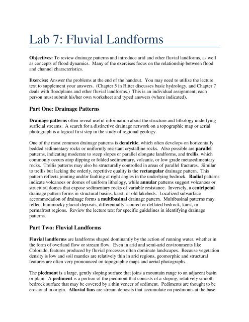
<strong>Lab</strong> 7: <strong>Fluvial</strong> <strong>Landforms</strong><br />
Objectives: To review drainage patterns and introduce arid and other fluvial landforms, as well<br />
as concepts of flood dynamics. Many of the exercises focus on the relationship between flood<br />
and channel characteristics.<br />
Exercise: Answer the problems at the end of the handout. You may need to utilize the lecture<br />
text to supplement your answers. (Chapter 5 in Ritter discusses basic hydrology, and Chapter 7<br />
deals with floodplains and other fluvial landforms.) This is an individual assignment; each<br />
person must submit his/her own worksheet and typed answers (where indicated).<br />
Part One: Drainage Patterns<br />
Drainage patterns often reveal useful information about the structure and lithology underlying<br />
surficial streams. A search for a distinctive drainage network on a topographic map or aerial<br />
photograph is a logical first step in the study of regional geology.<br />
One of the most common drainage patterns is dendritic, which often develops on horizontally<br />
bedded sedimentary rocks or uniformly resistant crystalline rocks. Also possible are parallel<br />
patterns, indicating moderate to steep slopes or parallel elongate landforms, and trellis, which<br />
commonly occurs atop dipping or folded sedimentary, volcanic, or low grade metasedimentary<br />
rocks. Trellis patterns may also be structurally controlled in areas of parallel fractures. Similar<br />
to trellis but lacking the orderly, repetitive quality is the rectangular drainage pattern. This<br />
pattern reflects jointing and/or faulting at right angles in the underlying bedrock. Radial patterns<br />
indicate volcanoes or domes of uniform lithology, while annular patterns suggest volcanoes or<br />
structural domes that expose sedimentary rocks of variable resistance. Inversely, a centripetal<br />
drainage pattern forms in structural basins, karst, or old lakebeds. Localized subsurface<br />
accommodation of drainage forms a multibasinal drainage pattern. Multibasinal patterns may<br />
reflect hummocky glacial deposits, differentially scoured or deflated bedrock, karst, or<br />
permafrost regions. Review the lecture text for specific guidelines in identifying drainage<br />
patterns.<br />
Part Two: <strong>Fluvial</strong> <strong>Landforms</strong><br />
<strong>Fluvial</strong> landforms are landforms shaped dominantly by the action of running water, whether in<br />
the form of overland flow or stream flow. Even in arid and semi-arid environments like<br />
Colorado, features produced by fluvial processes often dominate landscapes. Because vegetation<br />
density is low and soil mantles are relatively thin in arid regions, geomorphic and structural<br />
features are often very pronounced on topographic maps and aerial photographs.<br />
The piedmont is a large, gently sloping surface that joins a mountain range to an adjacent basin<br />
or plain. A pediment is a portion of the piedmont that consists of a sloping, relatively smooth<br />
bedrock surface that may be covered by a thin veneer of sediment. Pediments are thought to be<br />
erosional in origin. Alluvial fans are stream deposits that accumulate on piedmonts at the base
of mountain fronts. They are fan-shaped in plan-view and convex-up in a cross-section taken<br />
parallel to the mountain front. Fans are commonly dissected by distributary channels or washes,<br />
all of which are probably not active at any one time. The coalescing of several adjacent alluvial<br />
fans along a mountain front forms Bajadas. The transition from a series of single fans to a<br />
bajada is complete when the cone shape of each individual fan is lost.<br />
Bolsons are extensive, flat basins or depressions, almost or completely surrounded by mountains<br />
and from which drainage has no surface outlet. These arid region features characteristically have<br />
centripetal drainage patterns and commonly have level plains in their center called playas.<br />
Playa lakes may form during heavy rainfall, but are usually short-lived, due to aridity and<br />
consequent infiltration and evaporation.<br />
In areas of very different climates, some streams have a natural inclination to develop a sinuous<br />
or meandering channel pattern. The growth of a meander results from erosion of the outside<br />
bank of each bend and concurrent deposition of material on the inside of each curve. As the<br />
meander bend migrates laterally, the continued accretion of sediment on the inside of the<br />
meander curve forms a point bar. Meanders also migrate downstream because of more effective<br />
erosion occurring on the downstream side of the meander bend. Differential erosion causes these<br />
meander bends to become distorted and increasingly sinuous until a threshold of disequilibrium<br />
is reached. Once unstable, the river cuts across the meander loop to follow a more direct course.<br />
Abandonment of the old meander loop produces a crescent-shaped lake called an oxbow lake.<br />
Periodically, a stream will form temporary cutoff channels during high discharge without<br />
permanently altering the channel pattern. This process, coupled with continued lateral migration<br />
of a meander and point bar deposition, forms a series of low ridges and shallow swales on the<br />
inside of meander bends called ridge and swale topography or meander scroll topography.<br />
Floodplains are formed by a number of processes, but lateral channel migration and vertical<br />
overbank deposition are believed to be the most important processes in operation. Most<br />
floodplains form by the interaction of a number of processes; the relative importance of these<br />
processes varies from situation to situation.<br />
A natural levee forms when a river leaves the confines of its channel and deposits coarsegrained<br />
material adjacent to the bank edge. This coarse-grained material continues to<br />
accumulate, due to subsequent flooding, and a natural levee is formed. On topographic maps<br />
only large levees are visible. These levees are recognizable as elongate, narrow ridges adjacent<br />
to a channel.<br />
Occasionally, river flow breaches a levee, forming a gap in the levee called a crevasse.<br />
Sediment is deposited on the floodplain in a fan-shaped deposit of debris called a crevasse splay.<br />
These features tend to form on floodplains having well-developed levees which form barriers to<br />
surface drainage attempting to enter the river. These areas are called backswamps; they play an<br />
important role in reducing flood peaks downstream by trapping and temporarily storing<br />
floodwater, which has breached the levee.
Terraces are abandoned floodplains formed during a period when the river flowed at a<br />
topographically higher elevation. Terraces result when channel downcutting lowers a river’s<br />
level, creating a new – lower and smaller – floodplain. Terrace surfaces represent relic features<br />
that are no longer directly related to current flood hydrology. Terraces form in response to<br />
changes in stream discharge or bedload sediment transport rates.<br />
Many terraces classification systems based on different distinguishing criteria are currently in<br />
use. Genetic terms that explain the way in which terraces form include erosional terraces,<br />
which are created primarily by lateral erosion, and depositional terraces, which represent an<br />
uneroded surface of older channel fill. Another classification system divides terraces into<br />
tectonic and climatic terraces, based on the cause of terrace formation. More descriptive terms<br />
include strath (bedrock) and alluvial (fill) terraces. Similarly, paired terraces occur on both<br />
sides of the channel at equal elevations. These paired terraces are usually interpreted as former<br />
floodplain levels of similar age. Unpaired terraces, on the other hand, vary in elevation on<br />
either side of the channel. Unpaired terrace formation has been attributed to slow incision with<br />
slow lateral migration. Therefore, the unpaired terraces represent floodplain levels of different<br />
ages.<br />
Part Three: Hydrologic Concepts<br />
The floodplain is generally considered the flat surface adjacent to a channel. Floodplains are<br />
located at a slightly higher elevation than the channel and provide temporary storage of<br />
floodwaters. When water rises above the level of the banks, a portion of the discharge continues<br />
to flow downstream over the floodplain. Because the floodplain usually has many trees, bushes,<br />
houses, etc., the flow encounters more resistance than the water still flowing down the channel.<br />
Based on Manning’s equation (Ritter, Chapter 6), we know that water velocity is proportional to<br />
the channel slope (S 1/2 ), hydraulic radius (R 2/3 ), and the channel resistance (Manning’s n).<br />
Therefore, we can deduce that water traveling over the floodplain will generally travel more<br />
slowly than water traveling in the channel.<br />
As a flood-wave moves downstream, resistance in the channel and on the floodplain tends to<br />
slow the release of a portion of the water (flood attenuation). Given an overall volume of storm<br />
runoff, resistance to flow tends to decrease flood peaks downstream and lengthens the period of<br />
time necessary for the flood to pass a given location. The more resistance offered by the channel<br />
and the floodplain, the more dramatic the effects of flood attenuation become.<br />
To help demonstrate this process, you can picture all of your friends lining the side of a channel<br />
armed with buckets. As a flood-wave approaches, some of your friends fill their buckets from<br />
the channel and then pour the water back into the channel at a later point in time. If you are<br />
standing downstream from your friends, it will take a longer time for all of the flood water to<br />
reach you than it would have taken without the bucket storage (temporary floodplain storage). If<br />
more of your friends fill and empty their buckets (increased channel and floodplain resistance),<br />
then the flood-wave will take even longer to pass you (more attenuated flood-wave).<br />
Analyzing Flood Hydrographs
The flood hydrograph is a plot of stream discharge versus time. The hydrograph illustrates the<br />
rate of increase of river stage, the flood peak magnitude, the duration of high flow, and the rate<br />
of descent of river stage. The storm hydrograph has a plot of precipitation intensity and<br />
volume superimposed on the discharge hydrograph. This information allows one to determine<br />
the relationship between storm precipitation and the resultant rate of discharge at a stream gaging<br />
station. A typical hydrograph is illustrated in Figure 1.<br />
RUNOFF<br />
BASEFLOW<br />
PRECIPITATION (cm)<br />
Figure 1. Storm hydrograph shows the relationship between precipitation and stream discharge.<br />
The point of maximum discharge is called the flood peak or peak flow and corresponds with<br />
highest flood stage. The rising limb of the hydrograph is characteristically steeper than the<br />
falling or recession limb, reflecting the relatively rapid rate of transport of surface runoff to the<br />
channel and the relatively slow release of water held in storage and in groundwater storage.<br />
Stream discharge can be separated into two general components: 1) direct runoff or quickflow<br />
and 2) baseflow or delayed flow. Baseflow, derived primarily from groundwater flow, sustains<br />
stream flow during periods of low precipitation. Because hydrographs represents stream<br />
discharge over time, they include both baseflow and storm runoff (or direct runoff) components.<br />
Various methods can be used to separate the hydrograph; the particular method chosen in a given<br />
situation is largely arbitrary.<br />
The lag time is defined as the time interval between the center of mass of the storm precipitation<br />
and the center of mass of the flood hydrograph, represented by the peak (Figure 1). The<br />
precipitation hyetograph is usually plotted either on the left side of the hydrograph or in the<br />
upper left corner of the diagram to facilitate comparison between precipitation and discharge.<br />
Streams with short lag times are called flashy and represent situations where precipitation is<br />
delivered rapidly to the stream channel, presumably as direct runoff. As the volume of direct<br />
runoff increases, the magnitude of the flood peak increases. Moreover, the groundwater
component decreases when direct runoff is high because less water is available for groundwater<br />
recharge and baseflow discharge.<br />
The usefulness of the stream hydrograph in flood prediction and planning should be very<br />
apparent. Estimations of storm runoff volume and stream discharge are essential in effective<br />
flood planning and design of engineering structures, such as dams and levees. These values can<br />
be easily determined from the storm hydrograph.<br />
Rating Curves and Flood Frequencies<br />
Statistical probability analysis of discharge records (collected by the U.S. Geological Survey and<br />
other federal, state, and private agencies) forms the basis for flood frequency studies. These<br />
discharge records contain mean daily discharge and the maximum instantaneous flow for the<br />
year, as well as the corresponding gauge height for each gaging station. These data can be used<br />
to construct a rating curve, which is the graphical relationship between stage and discharge at a<br />
particular gaging station, and a flood frequency curve, which is a plot of discharge versus<br />
statistical recurrence interval on logarithmic graph paper.<br />
A rating curve is a plot on regular graph paper that relates stage to discharge for a given channel<br />
cross-section. The form of the rating curve is normally parabolic but may show some<br />
irregularities. A measure of the scatter of points about the best line fit determines the adequacy<br />
of a rating curve. Construction of a rating curve requires many discharge measurements, taken at<br />
a gaging site, that span a wide spectrum of discharge values. Naturally, the accuracy of the<br />
resultant rating curve is directly proportional to the number of available discharge and related<br />
stage measurements.<br />
The recurrence interval (RI) is the time scale used for flood frequency curves, plotted along<br />
the abscissa. The recurrence interval is defined as the average interval of time within which a<br />
discharge of a given magnitude will be equaled or exceeded at least once. There are two<br />
commonly used methods to manipulate discharge data for studying flood frequency. The first<br />
method is the annual-flood array, in which only the highest instantaneous peak discharge in a<br />
water year is recorded. The list of yearly peak flows for the entire period of a record are then<br />
arranged in order of descending magnitude, forming an array. The recurrence interval of any<br />
given flow event for the period of record can be determined by using the equation:<br />
RI<br />
=<br />
N + 1 ,<br />
M<br />
where:<br />
RI = recurrence interval,<br />
N = the total number of years in record, and<br />
M = the rank or magnitude of the flow event.<br />
Some hydrologists and geomorphologists object to the use of annual floods because this method<br />
uses only one flood in each year; occasionally, the second highest flood in a given year – which<br />
is omitted – may outrank many annual floods. The other method commonly used in flood<br />
frequency analysis is the partial-duration series. When using this method, all floods of greater<br />
magnitude than a pre-selected base are listed in an array, without regard to whether they occur
within the same year. As you might expect, this method also draws criticism. The main problem<br />
with the partial-duration series is that each included flood may not be a truly independent event<br />
(i.e., flood peaks counted as separate events may actually represent one period of flooding.)<br />
Because of the simplicity and general reliability of the annual-flood array, the U.S. Geological<br />
Survey has adopted this method.<br />
It is critical to note that the flood array method of flood frequency analysis is a probabilistic<br />
approach in which flood occurrences are treated as random events. The method assumes that all<br />
floods occurring during a period of time constitute a sample of an infinitely large population in<br />
time. Specifically, if in a period of 30 years of record the largest flood recorded was of a certain<br />
magnitude, it is probable that a flood of equal magnitude will occur within the next 30 years. It<br />
therefore follows that the accuracy of flood prediction will depend to a large degree on the length<br />
of time for which discharge records are available. Predicting a flood of a certain magnitude is a<br />
calculated risk based upon a statistical probability. There is an element of chance involved.<br />
Many times the flood record is much shorter than what we would desire. Often such records<br />
contain an individual flood whose recurrence interval is much greater than the total period of<br />
record. The point representing such an event will lie well off the general trend of the curve<br />
defined by the other points. Such an outlying point will cause the best-fit line to be shifted into a<br />
position that is unrepresentative of the actual scenario. This variability brings into question the<br />
validity of predicting rare flood events from a relatively short period of record. There is<br />
obviously a large degree of uncertainty in doing this, but frequently there are no alternatives.<br />
Despite these problems, flood frequency analysis remains the most accurate method of flood<br />
forecasting yet devised.<br />
Even when flood probability is determined from long periods of record, the recurrence interval is<br />
only the average frequency with which a given discharge will occur. The 100-year flood is not<br />
necessarily an event that will occur at 100-year intervals. Rather, there is a one-percent chance<br />
that the 100-year flood will occur in any given year. If one occurred in a given year, there is still<br />
a one-percent chance that it will occur again the following year. The probability that a flood<br />
with a given recurrence interval will occur or be exceeded in any year can be determined using<br />
the following equation:<br />
1<br />
p )<br />
RI<br />
n<br />
= 1−<br />
(1 − ,<br />
where:<br />
p = probability of occurrence,<br />
RI = recurrence interval of the event in question, and<br />
n = the number of years in question.<br />
For example, there is a four-percent chance that the 50-year flood will occur in the next two<br />
years because:<br />
1 2<br />
p = 1−<br />
(1 − ) *100 = 3.96 or 4%<br />
50
The mean annual flood is simply the arithmetic mean of all the maximum discharges in the<br />
annual array, and for most flood series distributions, it has been found to have a recurrence<br />
interval of 2.33 years. In fact, Dalrymple (1960) has defined the mean annual flood as the 2.33-<br />
year flood, as picked from the graphic flood frequency curve.<br />
The uncertainty of extrapolating a flood frequency curve, as well as the possible error introduced<br />
by fitting a curve through the peak discharge point distribution, make flood forecasting a risky<br />
venture. Hydrologists and geomorphologists must be aware of the limitations inherent in flood<br />
forecasting methods before making predictions.
<strong>Fluvial</strong> <strong>Landforms</strong><br />
<strong>Lab</strong> 7 Exercises<br />
Name __________________<br />
<strong>Lab</strong> Day ________________<br />
Mount Rainier, Washington<br />
1. (a) What drainage pattern is formed on Mount Rainier?<br />
(b) What does the drainage pattern indicate about the underlying structure and lithology of<br />
this mountain?<br />
Lake Wales, Florida<br />
2. What drainage pattern dominates this area?<br />
Strasburg, Virginia<br />
3. (a) What drainage pattern occurs in this region?<br />
(b) What do the erosional patterns of the channels indicate about the relative resistance of the<br />
ridges and valleys?<br />
St. Paul, Arkansas<br />
4. (a) What is the drainage pattern in this area?<br />
(b) Qualitatively describe the drainage density in this area.<br />
Bright Angel, Arizona<br />
5. (a) What drainage pattern occurs on the Kaibab Plateau?<br />
(b) What drainage pattern dominates Bright Angel Canyon?<br />
(c) What channel pattern best characterizes the Colorado River in Granite Gorge?
Manassa NE, Colorado<br />
6. (a) What drainage pattern occurs around Flat Top Mountain?<br />
(b) Qualitatively describe the drainage density around Flat Top Mountain.<br />
(c) What are the ponds in the northwest corner of the map?<br />
Brandon, Vermont<br />
7. (a) What is the fluvial landform represented by the wetlands along either side of Otter Creek?<br />
(b) What fluvial landform probably separates these wetlands from the river?<br />
Ennis, Montana<br />
8. (a) What type of channel pattern does the Madison River exhibit?<br />
(b) The Cedar Creek Alluvial Fan represents a large deposit of material transported from the<br />
local mountains. How could this alluvial fan be affecting the Madison River channel<br />
pattern?<br />
Guadalupe Peak, Texas<br />
9. (a) What geomorphic name would you apply to Salt Lake?<br />
(b) What is the gently sloping area linking Salt Basin and Crow Flats to the Guadalupe<br />
Mountains?<br />
Furnace Creek, California<br />
10. (a) What is the geomorphic name for the landform stretching from the northwestern corner of<br />
the quadrangle to the base of the quadrangle near the San Bernardino Meridian?<br />
(b) How could this landform have developed?
(c) What is the geomorphic name applied to Death Valley?<br />
Menan Buttes, Idaho<br />
11. What is the fluvial landform represented by the crescent shaped mounds along the inside of<br />
the meander bends?<br />
Menan Buttes, Idaho and Flaming Gorge Utah-Wyoming<br />
12. (a) The Snake River and Henry’s Fork located on the Menan Buttes, Idaho, topographic map<br />
and the Green River located on the Flaming Gorge, Utah-Wyoming, topographic map<br />
represent what channel pattern?<br />
(b) Based on the presence or lack of fluvial landforms and the relative incision of these<br />
channels, which of the above channels shows the most active lateral channel migration<br />
and why?<br />
(c) Which of these channels would tend to form levees and why?<br />
Cumberland, Maryland-Pennsylvania-West Virginia<br />
13. (a) What is the width of the floodplain (in kilometers) of Wills Creek near Lovers’ Leap (The<br />
Narrows)?<br />
(b) What is the width of the floodplain (in kilometers) of Wills Creek at Locus Grove?<br />
14. How would flood attenuation vary between these two reaches?
Flood Hydrology<br />
Answer the following questions using your knowledge of flood processes and fluvial landforms.<br />
Information can also be found in your lecture text and in this handout.<br />
Figure 1: Plan-view map of a natural river/floodplain system.
Figure 2: Runoff event at station A resulting from rain in the upper portion of the basin.<br />
Figure 3: Flood frequency curve for streamflow gaging station A.
Figure 4: Rating curve for station A.<br />
15. The streamflow-gaging station at point A records a runoff event for a short precipitation<br />
event occurring at time = 0 hours (Fig. 2).<br />
What is the lag-to-peak for this flow?<br />
16. Determine the peak discharge from the hydrograph and determine the approximate<br />
recurrence interval for this flow from the attached flood frequency curve (Fig. 3).<br />
17. What is the probability that a second flood of equal discharge will occur in the next 7 years?<br />
Show your work
18. You happen to be fishing at streamflow-gaging station A during this runoff event and you<br />
carefully observe the elevation of your fishing bobber during the runoff event. (The bobber<br />
remains at the same cross section and does not move downstream). Using the attached rating<br />
curve (Fig. 4) draw the elevation at the bobber at each one-hour increment from time = 2<br />
hours until time = 11 hours. (Plot on the attached graph 1). This plot is essentially the same<br />
graph that would be automatically recorded by the stage recorder inside the streamflowgaging<br />
station.
Predicted Flood and Channel Responses<br />
Use the Figures 1-4 to help you answer the following questions:<br />
Fig. 1 shows a plan-view map of a natural river/floodplain system.<br />
Fig. 2 records a runoff event at streamflow-gaging A resulting from rain in the upper<br />
portion of the basin.<br />
Fig. 3 is a flood frequency curve for this stream-flow gaging station.<br />
Fig. 4 is a rating curve for this station.<br />
19. Using your knowledge of flood attenuation, draw the approximate hydrograph that would be<br />
observed at streamflow-gaging station B for the same rainfall event recorded at streamflowgaging<br />
station A (Fig. 2).<br />
On the attached sheet, plot the Hydrograph for Streamflow-gaging Station B Pre-levee.<br />
Assume it takes approximately 3 hours for the first portion of the runoff to travel from gage<br />
A to gage B. Also assume there are no permanent water losses or inputs between the two<br />
stations.
20. Now we will assume that the town of Richville constructs the levee indicated on the map to<br />
protect their town from flooding. Estimate and draw a new hydrograph for streamflowgaging<br />
station B using the same original hydrograph for streamflow-gaging station A.<br />
On the attached sheet, plot the Hydrograph for Streamflow-gaging Station B Post-levee.<br />
Assume there are no permanent water losses or inputs between the two stations.<br />
21. In a short typed paper discuss what effects the levee will have on the flood hydrograph at<br />
streamflow-gaging station B. In particular, try to address the following questions: How will<br />
the levee affect the volume of storm runoff, flood peak and time-to-peak of the flood?<br />
(Describe qualitatively.) If there were no changes in the dimensions of the channel at<br />
streamflow-gaging station B, would a rating curve for this station need to be adjusted?<br />
(Indicate why or why not.) Would a pre-levee flood frequency curve for station B need to be<br />
adjusted? (Indicate why or why not.) If you lived a small elevation above the river near<br />
station B, what long-term effects could the levee have on your property value? (Think about<br />
the elevation and frequency of flooding.)