Aggregate Planning - PageOut
Aggregate Planning - PageOut
Aggregate Planning - PageOut

Create successful ePaper yourself
Turn your PDF publications into a flip-book with our unique Google optimized e-Paper software.
OPERATIONS MANAGEMENT<br />
<strong>Aggregate</strong> <strong>Planning</strong><br />
Learning Objectives<br />
• Explain business, sales & operations planning<br />
• Identify different aggregate planning strategies<br />
• Identify options for changing demand & capacity<br />
• Develop aggregate plans & calculate costs<br />
• Evaluate the impact of aggregate plans on functional<br />
areas<br />
• Describe the differences between plans for services &<br />
manufacturing companies<br />
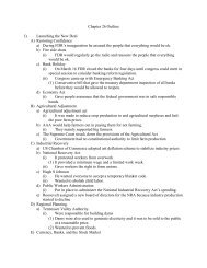
Long<br />
Range<br />
Operations <strong>Planning</strong> Hierarchy<br />
Process <strong>Planning</strong><br />
Strategic Capacity <strong>Planning</strong><br />
Medium<br />
<strong>Aggregate</strong> <strong>Planning</strong><br />
Range<br />
Manufacturing<br />
Master Production Scheduling<br />
Services<br />
Material Requirements <strong>Planning</strong><br />
Short<br />
Range<br />
Order Scheduling<br />
Weekly Workforce &<br />
Customer Scheduling<br />
Daily Workforce &<br />
Customer Scheduling<br />
4
Business <strong>Planning</strong> Hierarchy<br />
Sales and Operations <strong>Planning</strong><br />
• Medium-term functional plans designed to<br />
operationalize the long-term strategic plan:<br />
• Marketing plan: defines the target customers<br />
• <strong>Aggregate</strong> production plan: identifies the desired<br />
inventory levels & staffing<br />
• Financial plan: identifies the source of funds, cash flows,<br />
& sets budgets<br />
• Engineering plan: explores needed product & process<br />
changes in support of the marketing plan<br />
<strong>Aggregate</strong> <strong>Planning</strong><br />
• Based on composite (representative)<br />
products:<br />
• Simplifies calculations<br />
• Forecasts for grouped items are more accurate<br />
• Considers trade-offs between holding<br />
inventory & short-term capacity based on<br />
workforce
Master Production Schedule<br />
• Breaks apart the composite product used in<br />
<strong>Aggregate</strong> <strong>Planning</strong>:<br />
• Identifies specific product configurations,<br />
quantities & dates<br />
• Used by marketing to determine units available<br />
to promise to customers<br />
<strong>Planning</strong> Approaches<br />
• Reactive approach:<br />
• Allow volume forecasts based on Marketing plan<br />
to drive production planning<br />
• Proactive approach:<br />
• Coordinate Marketing & Production plans to<br />
level demand using advertising & price<br />
incentives<br />
Inputs to / Outputs of<br />
<strong>Aggregate</strong> <strong>Planning</strong><br />
Inputs<br />
• A forecast of aggregate demand over planning horizon<br />
• Available Resources (current workforce, inventory levels,<br />
production rates, available capital etc.)<br />
• Alternative means available to adjust capacity and<br />
associated costs<br />
Outputs<br />
• A production plan: aggregate decisions concerning<br />
workforce,production, inventory levels + Cost of the plan
Demand-based Options<br />
• Finished goods inventories:<br />
• Anticipate demand, i.e….<br />
• Back orders & lost sales:<br />
• Delay delivery or allow demand to go unfilled<br />
• Shift demand to off-peak times:<br />
• Less inventory,<br />
• Proactive marketing, i.e. …<br />
Capacity-based Options<br />
• Overtime: Short-term option –Downside?<br />
• Pay workers a premium to work longer hours<br />
• Undertime: Short-term option – Why?<br />
• Slow the production rate or send workers home early<br />
(lowers labor productivity, but doesn’t tie up capital in<br />
finished good inventories)<br />
• Subcontracting: Medium-term option (cost, control)<br />
• Hire & fire workers: Long-term option<br />
• Change the size of the workforce (expensive?)<br />
Costs in <strong>Aggregate</strong> <strong>Planning</strong><br />
• Smoothing costs (i.e. hiring/firing costs)<br />
• Holding costs<br />
• Backordering costs<br />
• Regular time costs<br />
• Overtime costs<br />
• Subcontracting costs<br />
• Idle time costs
Techniques for AP<br />
• Informal or Trial-and-Error techniques<br />
• Most commonly used in practice.<br />
• Consist of developing simple tables and graphs that enable planners<br />
to visually compare projected demand requirements with existing<br />
capacity.<br />
• May not result in optimal aggregate plan.<br />
• Mathematical Techniques<br />
• Linear Programming<br />
• Simulation<br />
Strategies for Meeting Demand<br />
• Pure Strategies: Focused strategies<br />
• Level Strategy: constant level of production, variations in demand<br />
absorbed by some combination of capacity and demand based options<br />
• Chase Strategy: match production to the demand for every period<br />
• Mixed Strategies: Some combination of pure strategies.<br />
• Choice of strategy depends on:<br />
• company policy: e.g. no layoffs, subcontracting etc.<br />
• costs: match demand and supply within constraints imposed on them<br />
by policies or agreements and at minimum costs.
Pure Strategies<br />
• Level Strategy:<br />
• Use a constant workforce & produce similar quantities each time<br />
period.<br />
• Use inventories & backorders to absorb demand peaks & valleys.<br />
• Employee benefit from stable work hours.<br />
• Risk of rendering inventoried products obsolete.<br />
• Chase Strategy:<br />
• Match the production rate to the order rate by hiring and laying off<br />
employees as the order rate varies.<br />
• Minimize finished good inventories by trying to keep pace with<br />
demand fluctuations.<br />
• Low backlogs --> employees feel compelled to slow down out of<br />
fear of being laid off as soon as existing orders are completed.<br />
Mixed Strategies<br />
• Use a combination of options:<br />
• Build-up inventory ahead of rising demand &<br />
use backorders to level extreme peaks<br />
• Layoff or furlough workers during lulls<br />
• Subcontract production or hire temporary<br />
workers to cover short-term peaks<br />
• Reassign workers to preventive maintenance<br />
during lulls<br />
Developing <strong>Aggregate</strong> <strong>Planning</strong><br />
• Choose the basic strategy:<br />
• Level, chase, or hybrid<br />
• Determine the production rate:<br />
• Level plan with back orders: rate = average<br />
demand over the planning horizon<br />
• Level plan without back orders: rate is set to meet<br />
all demand on time<br />
• Chase plan: assign regular production, amount of<br />
overtime & subcontracted work to meet demand
Developing <strong>Aggregate</strong> <strong>Planning</strong>-Contd.<br />
• Calculate the size of the workforce needed<br />
• Calculate period-to-period inventory levels,<br />
shortages, expected hiring & firings, and overtime<br />
• Calculate period-by-period costs, then sum for<br />
total costs of the plan<br />
• Evaluate the plan’s impact on customer service<br />
and human resource issues<br />
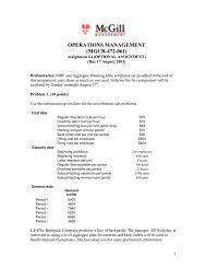
Example<br />
Example<br />
Plan A: LEVEL <strong>Aggregate</strong> Plan, Inventories and Back Orders<br />
Plan A: LEVEL <strong>Aggregate</strong> Plan, Inventories and Back Orders<br />
Period 1 2 3 4 5 6 7 8 Total<br />
Demand (units) 1,920 2,160 1,440 1,200 2,040 2,400 1,740 1,500 14,400<br />
Cumulative Demand 1,920 4,080 5,520 6,720 8,760 11,160 12,900 14,400<br />
Period Production 1,800 1,800 1,800 1,800 1,800 1,800 1,800 1,800 14,400<br />
Cumulative Production 1,800 3,600 5,400 7,200 9,000 10,800 12,600 14,400<br />
Ending Inventory 480 240 720<br />
Back Orders 120 480 120 360 300 1,380<br />
Total Cost Calculation for Plan A<br />
Regular-time Labor Cost<br />
$12.50 per hour x 160 hours per period x 8 periods x 90 employees $ 1,440,000<br />
Inventory Holding Cost<br />
720 units x $10 per unit $ 7,200<br />
Back-order Costs<br />
1,380 units x $25 per unit $ 34,500<br />
Total Costs $ 1,481,700
Example<br />
Plan B: LEVEL <strong>Aggregate</strong> Plan, Inventories and NO Back Orders, All<br />
Demand Met<br />
Plan B: LEVEL <strong>Aggregate</strong> Plan, Inventories and NO Back Orders, All Demand Met<br />
Period 1 2 3 4 5 6 7 8 Total<br />
Demand (units) 1,920 2,160 1,440 1,200 2,040 2,400 1,740 1,500 14,400<br />
Cumulative Demand 1,920 4,080 5,520 6,720 8,760 11,160 12,900 14,400<br />
Cum. Demand / # of Periods 1,920 2,040 1,840 1,680 1,752 1,860 1,843 1,800<br />
Period Production 2,040 2,040 2,040 2,040 2,040 2,040 2,040 2,040 16,320<br />
Cumulative Production 2,040 4,080 6,120 8,160 10,200 12,240 14,280 16,320<br />
Ending Inventory 120 - 600 1,440 1,440 1,080 1,380 1,920 7,980<br />
Total Cost Calculation for Plan B<br />
Regular-time Labor Cost<br />
$12.50 per hour x 160 hours per period x 8 periods x 90 employees $ 1,632,000<br />
Inventory Holding Cost<br />
7980 units x $10 per unit $ 79,800<br />
Hiring Costs<br />
12 employees x $800 $ 9,600<br />
Total Costs $ 1,721,400<br />
Example<br />
Plan C: CHASE <strong>Aggregate</strong> Plan, Using Hiring and Firing<br />
Plan C: CHASE <strong>Aggregate</strong> <strong>Planning</strong> ,Using Hiring and Firing<br />
Period 1 2 3 4 5 6 7 8 Total<br />
Demand (units) 1,920 2,160 1,440 1,200 2,040 2,400 1,740 1,500 14,400<br />
Employees Needed 96 108 72 60 102 120 87 75 720<br />
Number of Hires 6 12 42 18 78<br />
Number of Fires 36 12 33 12 93<br />
Total Cost Calculation for Plan C<br />
Regular-time Labor Cost<br />
$12.50 per hour x 160 hours per period x 720 employees $ 1,440,000<br />
Firing Costs<br />
93 employees x $500 each $ 46,500<br />
Hiring Costs<br />
78 employees x $800 each $ 62,400<br />
Total Costs $ 1,548,900<br />
Example<br />
Plan D: Hybrid <strong>Aggregate</strong> Plan, Initial Workforce and<br />
Overtime as Needed<br />
Plan D: Hybrid <strong>Aggregate</strong> Plan, Initial Workforce and Overtime as Needed<br />
Period 1 2 3 4 5 6 7 8 Total<br />
Demand (units) 1,920 2,160 1,440 840 1,080 1,680 1,620 1,500 14,400<br />
Regular time units produced 1,800 1,800 1,800 1,800 1,800 1,800 1,800 1,800 14,400<br />
Overtime units produced 120 360 480<br />
Ending Inventory - - 360 960 720 120 180 480 2,820<br />
Total Cost Calculation for Plan D<br />
Regular-time Labor Cost<br />
$12.50 per hour x 160 hours per period x 8 periods x 90 employees $ 1,440,000<br />
Overtime Labor Hours<br />
$18.75 per hour x 8 hours per unit x 480 units $ 72,000<br />
Holding Costs<br />
2,820 units x $10 per unit $ 28,200<br />
Total Costs $ 1,540,200
Master Scheduling Process<br />
• Master Schedule: Result of disaggregating the AP. It<br />
shows the quantity and timing of individual products over<br />
a shorter horizon<br />
Inputs<br />
Beginning inventory<br />
Master<br />
Forecast<br />
scheduling<br />
Customer orders (committed)<br />
Outputs<br />
Master production schedule<br />
Projected inventory<br />
Uncommitted inventory<br />
This schedule is used to determine material and inventory<br />
requirements for all the parts in the product (MRP)<br />
Master Scheduling Process<br />
• Done on an ongoing basis using time fences:<br />
6+ wks<br />
1-2 wks<br />
No Change<br />
Frozen<br />
2-4 wks<br />
+/- 5%<br />
Firm<br />
4-6 wks<br />
+/- 10% +/- 20%<br />
Full<br />
Open<br />
Non-Financial Criteria<br />
• Operations perspective:<br />
• Can operations ramp up & back down this quickly?<br />
• Much more difficult to accomplish<br />
• Human resources perspective:<br />
• Will employees tolerate being hired & fired so rapidly?<br />
• What about training & learning curve issues?<br />
• Marketing perspective:<br />
• All demand is met (assuming no strikes)
Service <strong>Planning</strong> Issues<br />
• Intangible products can’t be inventoried<br />
• Possible approaches:<br />
• Try to proactively shift demand away from peaks<br />
• Use overtime or subcontracting to handle peaks<br />
• Allow lost sales<br />
OPERATIONS MANAGEMENT<br />
Materials Requirement<br />
<strong>Planning</strong><br />
Learning Objectives<br />
• Distinguish independent & dependent demand<br />
• Describe the objectives & inputs of MRP<br />
• Explain MRP operating logic<br />
• Describe bill of materials & product structure trees<br />
• Understand the impact of lot size rules<br />
• Understand capacity requirements planning<br />
• Introduce advanced planning systems
Review: Types of Inventory<br />
Types of Demand<br />
• Independent:<br />
• Effects inventories that are managed separately from<br />
other items (e.g.: finished goods made-to-stock)<br />
• Demand is managed based on forecasts<br />
• Dependent:<br />
• Effects inventories that are managed to support<br />
production of other items (e.g.: component parts)<br />
• Demand is managed based on plans (e.g.: MPS)<br />
• Dependent items are needed just prior to when<br />
they are needed for production<br />
Demand is lumpy<br />
Little or no safety stock<br />
Independent Demand<br />
Dependent Demand<br />
Demand<br />
Stable demand<br />
Demand<br />
“Lumpy” demand<br />
Amount on hand<br />
Safety stock<br />
Time<br />
Time<br />
Amount on hand<br />
Time<br />
Time
Material Requirements<br />
<strong>Planning</strong><br />
• An information system that uses the concept of<br />
backward scheduling to push the right material,<br />
in the right amount, at the right time, into the<br />
production process<br />
• Used in dependent demand environments<br />
MRP Overview<br />
• Inputs:<br />
• Master production schedule<br />
• Bill of Materials<br />
• Inventory Records<br />
• Primary objectives:<br />
• Schedule of replenishment orders (timing & quantities of<br />
material requirements)<br />
• Maintain priorities & track performance to plan (changes<br />
in requirements and customer orders)
Overview<br />
Definitions<br />
• End item:<br />
• The product sold as a completed item or repair part (an<br />
independently demanded item)<br />
• Parent items:<br />
• Items produced from one or more “children”<br />
• Components:<br />
• Raw materials & other items (“children”) that are part of<br />
a larger assembly<br />
• MRP converts the production plan for final products into<br />
requirements for component items and raw materials:<br />
• What is needed?<br />
• When is needed?<br />
• How much is needed?<br />
When should procurement, fabrication assembly start for<br />
completing end items on time<br />
Procurement of<br />
raw material D<br />
Procurement of<br />
raw material F<br />
Procurement of<br />
raw material G<br />
Fabrication<br />
of part E<br />
Procurement of<br />
part C<br />
Procurement of<br />
part H<br />
Subassembly A<br />
Subassembly B<br />
Final assembly<br />
and inspection<br />
1 2 3 4 5 6 7 8 9 10 11
Lot Sizing Rules<br />
• Rules are used to change the frequency of<br />
replenishment orders & set the quantity of<br />
each order (balance holding & ordering costs<br />
to reduce total costs)<br />
• Common rules:<br />
• Fixed Order Quantity (FOQ)<br />
• Lot-for-Lot (L4L)<br />
• Periodic Order Quantity (POQ)<br />
End Item Example: Pie Safe<br />
Bill of Material (BOM)<br />
• A list of all the assemblies, components, &<br />
raw materials required to produce the end<br />
item<br />
Part Number<br />
Description Quantity Required<br />
PS1001-U Unfinished pie safe 1<br />
PSF1001-U Frame assembly 1<br />
PST 1001-U Cabinet top 1<br />
PSD 1001-U Door assembly 2<br />
PSD 1001-D Pre-cut door 1<br />
PSD 1001-I Punched tin insert 3<br />
PSD 1001-K Knob 1<br />
PSC 1001-U Closure assembly 1<br />
PSH 1001-U Hinge 4
Product Structure Tree<br />
• A graphical view of the BOM:<br />
Inventory Record<br />
• Gross requirements:<br />
• The total period demand for the item<br />
• Scheduled receipts:<br />
• An open order with an assigned due date<br />
• Projected available:<br />
• The projected inventory balance for the period<br />
• Planned orders:<br />
• Quantities & released dates suggested by the MRP<br />
system<br />
Example<br />
Inventory Record for Pie Safe<br />
Item: Pie Safe<br />
Lot size rule: L4L<br />
Lead time: 1 week<br />
0 1 2 3 4 5 6 7 8 9 10 11 12<br />
Gross requirements 0 0 0 100 0 0 100 0 0 100 0 0<br />
Scheduled receipts 100 100<br />
A Time Bucket<br />
100<br />
Projected available 0 0 0 0 0 0 0 0 0 0 0 0 0<br />
Planned orders 100 100 100
Operating Logic<br />
• Explosion:<br />
• Calculate the children’s time-phased gross<br />
requirements by multiplying the parent item’s<br />
planned order amount by the number of children<br />
required to produce one parent item<br />
Example<br />
Item: Pie Safe<br />
Lot size rule: L4L<br />
Lead time: 1 week<br />
0 1 2 3 4 5 6 7 8 9 10 11 12<br />
Gross requirements 0 0 0 100 0 0 100 0 0 100 0 0<br />
Scheduled receipts 100 100 100<br />
Projected available 0 0 0 0 0 0 0 0 0 0 0 0 0<br />
Planned orders 100 100 100<br />
Item: Hinge assembly<br />
Parent item: Pie Safe<br />
Lot size rule: FOQ = 800<br />
Children: None<br />
Lead time: 3 weeks<br />
0 1 2 3 4 5 6 7 8 9 10 11 12<br />
Gross requirements 0 0 400 0 0 400 0 0 400 0 0 0<br />
Scheduled receipts 800<br />
Projected available 700 700 700 300 300 300 700 700 700 300 300 300 300<br />
Planned orders 800<br />
Pie Safe Example<br />
Inventory Record for Pie Safe<br />
Item: Pie Safe<br />
Lot size rule: L4L<br />
Lead time: 1 week<br />
0 1 2 3 4 5 6 7 8 9 10 11 12<br />
Gross requirements 0 0 0 100 0 0 100 0 0 100 0 0<br />
Scheduled receipts 100 100 100<br />
Projected available 0 0 0 0 0 0 0 0 0 0 0 0 0<br />
Planned orders 100 100 100
Pie Safe Example- contd.<br />
First Inventory Record For Frame Assembly<br />
Item: Frame Assembly Parent: Pie Safe<br />
Lot Size Rule: FOQ=144 Children: None<br />
Lead Time: 3 weeks<br />
1 2 3 4 5 6 7 8 9 10 11 12<br />
Gross Requirements 0 0 100 0 0 100 0 0 100 0 0 0<br />
Scheduled Receipts<br />
Projected Available (120) 120 120 20 20 20 -80<br />
Planned Orders<br />
Pie Safe Example- contd.<br />
Updated Inventory Record For Frame Assembly<br />
Item: Frame Assembly Parent: Pie Safe<br />
Lot Size Rule: FOQ=144 Children: None<br />
Lead Time: 3 weeks<br />
1 2 3 4 5 6 7 8 9 10 11 12<br />
Gross Requirements 0 0 100 0 0 100 0 0 100 0 0 0<br />
Scheduled Receipts<br />
Projected Available (120) 120 120 20 20 20 64 64 64 108 108 108 108<br />
Planned Orders 144 144<br />
Pie Safe Example- contd.<br />
Updated Inventory Record For Door Assembly<br />
Item: Door Assembly Parent: Pie Safe<br />
Lot Size Rule: L4L Children: Pre-cut Door, punched tin insert, knob<br />
Lead Time: 1 week<br />
1 2 3 4 5 6 7 8 9 10 11 12<br />
Gross Requirements 0 0 200 0 0 200 0 0 200 0 0 0<br />
Scheduled Receipts<br />
Projected Available (0) 0 0 0 0 0 0 0 0 0 0 0 0<br />
Planned Orders 200 200 200
Pie Safe Example- contd.<br />
Inventory Record For Knob<br />
Item: Knob Parent: Door Assembly<br />
Lot Size Rule: FOQ=300 Children: none<br />
Lead Time: 2 weeks<br />
1 2 3 4 5 6 7 8 9 10 11 12<br />
Gross Requirements 0 200 0 0 200 0 0 200 0 0 0 0<br />
Scheduled Receipts<br />
Projected Available (250) 250 50 50 50 150 150 150 250 250 250 250 250<br />
Planned Orders 300 300<br />
Comparison of Lot Size Rules<br />
• Different rules yield to different replenishment order frequencies and<br />
order quantities.<br />
Inventory Record Pie Safe<br />
Item: Pie Safe Parent: None<br />
Lot Size Rule: FOQ=144 Children:Frame A., Top, Door A., Hinge kit, Closure Assembly<br />
Lead Time: 1 week<br />
1 2 3 4 5 6 7 8 9 10 11 12 13<br />
Gross Requirements 0 25 25 40 40 0 60 60 60 0 60 60 60<br />
Scheduled Receipts<br />
Projected Available (0) 0 119 94 54 14 14 98 38 122 122 62 2 86<br />
Planned Orders 144 144 144 144<br />
Comparison of Lot Size Rules<br />
Inventory Record Pie Safe<br />
Item: Pie Safe Parent: None<br />
Lot Size Rule: L4L Children:Frame A., Top, Door A., Hinge kit, Closure Assembly<br />
Lead Time: 1 week<br />
1 2 3 4 5 6 7 8 9 10 11 12 13<br />
Gross Requirements 0 25 25 40 40 0 60 60 60 0 60 60 60<br />
Scheduled Receipts<br />
Projected Available (0) 0 0 0 0 0 0 0 0 0 0 0 0 0<br />
Planned Orders 25 25 40 40 60 60 60 60 60 60<br />
Inventory Record Pie Safe<br />
Item: Pie Safe Parent: None<br />
Lot Size Rule: POQ=4 periods Children:Frame A., Top, Door A., Hinge kit, Closure Assembly<br />
Lead Time: 1 week<br />
1 2 3 4 5 6 7 8 9 10 11 12 13<br />
Gross Requirements 0 25 25 40 40 0 60 60 60 0 60 60 60<br />
Scheduled Receipts<br />
Projected Available (0) 0 105 80 40 0 0 120 60 0 0 120 60 0<br />
Planned Orders 130 180 180
Comparison of Lot Size Rules<br />
Total Cost= Holding Cost + Ordering Cost<br />
H=$0.10 per period per unit, S= $25 per order<br />
• Fixed Order Quantity (FOQ)<br />
825x($0.10)+4x($25)=$182.5<br />
• Lot-for-Lot (L4L)<br />
0x($0.10)+10x($25)=$250.0<br />
• Periodic Order Quantity (POQ)<br />
585x($0.10)+3x($25)=$133.50<br />
MRP Outputs<br />
Primary Reports<br />
• Planned orders - schedule indicating the amount and timing of future<br />
orders.<br />
• Order releases - Authorization for the execution of planned orders.<br />
• Changes - revisions of due dates or order quantities, or cancellations of<br />
orders.<br />
Secondary Reports<br />
Performance-control reports - Assess performance<br />
<strong>Planning</strong> reports - Assess future material<br />
requirements.<br />
Exception reports - Calls attention to major<br />
discrepancies.
Shortcomings of MRP<br />
• Uncertainty: not taken into account.<br />
• Capacity: till now mostly uncapacitated.<br />
• Nervousness: major changes in production plan due to<br />
revised schedule.<br />
Capacity Requirements<br />
<strong>Planning</strong> (CRP)<br />
• Similar to rough cut capacity planning<br />
• CRP is a feasibility check on labor &<br />
machine utilization:<br />
• Compare the open orders & planned orders<br />
(from the MRP) to the actual shop floor capacity<br />
Example
Advanced <strong>Planning</strong> Systems<br />
• Manufacturing Resource <strong>Planning</strong> (MRP II):<br />
• Second generation MRP systems that connect to<br />
financial systems & help synchronize internal<br />
operations<br />
• Enterprise Resource <strong>Planning</strong> (ERP):<br />
• An information system designed to integrate<br />
internal & external processes of a supply chain<br />
via a centralized database<br />
ERP Overview