Practice Final Exam – STCC204 The following are the ... - Statistics

Practice Final Exam – STCC204
The following are the types of questions you can expect on the final exam. There are 24 questions on this practice
exam, so it should give you a good indication of the length of the exam. On the final exam the 25 th question will be
“Turn in your crib sheet with your exam paper”. With only 24 questions, it is not possible to address all of the
topics we covered. You need to study your other assignments and lecture notes to be sure you have studied
adequately. Note: Copies of the t-distribution, chi square distribution and control chart constants will be provided
with the exam.
1. The basic components of a time series model are
a. time, control, sampling, and inference
b. trend, control, seasonal, and inference
c. trend, cyclic, seasonal, and irregular
d. time, control, seasonal, and irregular
e. time, cyclic, seasonal, and irregular
2. Up or down movements in a time series that are related to specific times of the year would be reflected in the
____________ component of a time series.
a. trend;
b. cyclic;
c. seasonal;
d. irregular;
e. bias.
3. A linear trend was detected for Y, electrical power consumption for the years 1991 (t=1) to 2000 (t=10). The
least squares equation obtained for the trend is Y′ = 105.3 + 20.7t. Forecast the value for 2001.
a. 319.1
b. 212.3
c. 126.0
d. 333.0
4. For the following time series data, compute the five period moving average for time t = 9.
t 1 2 3 4 5 6 7 8 9 10 11 12
Y t 28 21 27 32 36 31 43 42 50 48 51 50
a. 39.8
b. 46.8
c. 48.67
d. 46.67
e. 50.0
5. If there is a very strong linear relationship between two quantitative variables then the correlation coefficient
must be
a. close to 1
b. close to -1
c. Either (a) or (b)
d. None of the above.
6. If the coefficient of determination is 0.81, what percent of variation is not explained?
a. 19%
b. 90%
c. 66%
d. 81%
e. None of the above

7. The term extrapolation refers to
a. using the sample regression equation to predict or estimate a value of Y using a value for X that is not within
the range of the X-values in the sample.
b. using a straight line regression equation to represent data that show a non-linear relationship between the two
variables.
c. using a least squares regression equation when the residuals are not normally distributed
d. using a regression equation when the sub-populations of Y-values do not have equal standard deviations.
e. None of the above.
8. The measure that indicates the amount of dispersion of the observed values about the regression line is denoted
a. s Y·X
b. Y′
c. a
d. b
e. None of the above
9. In regression analysis, which of the following is not a required assumption?
a. The means of the sub-populations of Y-values all fall on a line.
b. The standard deviations of the sub-populations are all equal.
c. The Y-values are independent.
d. The sub-populations are normally distributed.
e. All of the above are required assumptions.
10. An economist wanted to investigate the relationship between monthly long distance phone charges and monthly
income. He collected data for last month from a simple random sample of 40 households in the Denver area. In
particular, he recorded the long distance phone charges for that month (Y) and the monthly income (X). The
economist computed a regression equation and a correlation coefficient. Residuals were computed to check the
regression assumptions. These residuals are
a. differences between the observed monthly income and the predicted monthly income using the regression
equation
b. the difference between the observed degrees of freedom and the actual degrees of freedom
c. the values obtained by predicting the long distance phone charges for each monthly income observed in the
sample
d. the values obtained by computing a prediction interval for each monthly income observed in the sample
e. differences between the observed long distance charges and the charges predicted using the regression equation
11. A regression model was fit to predict bear age using weight as the independent variable and the Minitab output
is shown below. Based on this output, what can be concluded about the correlation between age and weight?
The regression equation is
Age = 2.61 + 0.219 Weight
Predictor Coef SE Coef T P
Constant 2.613 4.408 0.59 0.555
Weight 0.21912 0.01992 11.00 0.000
S = 21.68 R-Sq = 59.9% R-Sq(adj) = 59.4%
a. The correlation is positive.
b. The correlation is negative.
c. The correlation is equal to 0.599
d. The correlation is equal to 0.219.
e. Age and weight are weakly correlated.

12. A regression model was fit to predict bear age using weight as the independent
variable. A residual plot is shown here. Based on this plot, we can conclude that
the following assumption of regression is violated
a. For each value of X, there is a group of Y values, and these Y value are normally
distributed.
b. The means of the normal distributions of the Y values all lie on the straight line
of regression.
c. The standard deviations of these normal distributions are equal.
d. The Y values are statistically independent.
e. This is impossible to determine without knowing the sample size.
Residual
80
60
40
20
0
-20
-40
0
Residuals Versus the Fitted Values
(response is Age)
50
100
Fitted Value
13. A study was performed to investigate the strength of the linear relationship between Y, square footage of a home and X,
the income of the residents. A sample of 10 homes was obtained, resulting in a correlation coefficient equal to 0.843. In
testing at the .01 significance level whether or not there is a linear relationship between Y and X, the decision would be
a. Reject H 0 , since t > 2.896 or t 3.355 or t 4.432 or t 2.764 or t 3.169 or t

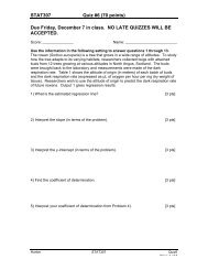
17. A food company uses filling machines to package 12 ounce boxes of a certain type of breakfast cereal. The
variability in this process is due to chance causes only. This process is said to be
a. changable
d. in control
b. assignable
e. None of the above.
c. out of control
18. The owner of a grounds-keeping service wants to identify the reasons why past clients discontinued service
with his company. Given below is a Pareto chart for data the owner collected from clients who discontinued
service in the past year. The categories are:
1-too expensive
2-dissatisfied with quality of service
3-moved
4-too many missed appointments
5-other
Based on this chart, which of the following
statements are true for the 39 clients
represented in the chart?
1) Expense is the most frequent
reason for discontinuing service.
2) Customer dissatisfaction with
service accounts for 71.8% of the
reasons for discontinuing sevice.
3) The “other” category accounts for
the largest percentage of the
reasons for discontinuing service.
a. 1,2 and 3
b. 2 only
c. 1 and 2
d. 1 and 3
e. 1 only
Count
40
30
20
10
0
Defect 1 2 3 4 5
Count
Percent
Cum %
Pareto Chart for Defect
16 12 5 3 3
41.0 30.8 12.8 7.7 7.7
41.0 71.8 84.6 92.3 100.0
19. In a production process, four items were sampled every hour to set up a control chart for the process. The
initial information obtained is shown below.
Measurement
Time 1 2 3 4
9 a.m. 1.0 4.0 5.0 2.0
10 a.m. 2.0 3.0 2.0 1.0
11 a.m. 1.0 7.0 3.0 5.0
What are the control limits for the mean chart?
a. 5.916 and 0
b. 5.916 and 0.084
c. 0.729 and 3.0
d. 3.0 and 4.0
20. The manufacturing of circuit boards involves a process in which gold plating is placed on each board. To
monitor the thickness of the gold plating on the circuit boards, ten samples of 4 gold plating thickness
measurements were obtained. Using these ten samples, an R-chart was obtained. All of the points on the R-chart
fell between the control limits, and the chart showed no pattern. What can be said regarding the variability of the
process, based on the control chart?
a. The process is in control.
b. The process is not in control.
c. Nothing can be determined, since the chart is not appropriate for investigating variability.
d. Nothing can be determined, since the chart is not used for quality control.
100
80
60
40
20
0
Percent

21. Which of the following is not true about the chi square distribution when used to test whether two qualitative variables are
related.
a. It is based on the sample size.
b. It is non-negative.
c. It is positively skewed.
d. When degrees of freedom change a new distribution is created.
22. A small college offers students complete freedom of choice when registering for courses. This semester there were seven
sections of a particular mathematics course. The sections were scheduled to meet at various times with a variety of instructors.
The table below shows the number of students who selected each of the seven sections. Do the data indicate that the students
had a preference for certain sections, or do they indicate that each section was equally likely to be chosen? Note: The
calculated value for the test statistic equals 12.94. Use a .10 significance level.
Section
1 2 3 4 5 6 7 Total
Number of Students 18 12 25 23 8 19 14 119
a. Fail to reject H 0 and conclude that class sections are not equally likely.
b. Fail to reject H 0 and conclude that class sections could be equally likely.
c. Reject H 0 and conclude that class sections are not equally likely.
d. Reject H 0 and conclude that class sections could be equally likely.
23. A video store chain in Colorado wishes to compare movie preferences for men and women. A random sample of 350
video store customers were asked what type of movie they most preferred. The responses are listed in the following
contingency table.
Comedy Adventure Drama Horror Sci-Fi Total
Men 34 35 26 25 74 194
Women 35 17 57 25 22 156
Total 69 52 83 50 96 350
Compute the expected frequency for women who prefer drama, when testing whether movie preference and gender are related.
a. 57.00
b. 41.29
c. 36.99
d. 46.65
e. None of the above.
24. For the above problem, the following results were obtained using Minitab:
Chi-Sq = 0.471 + 1.324 + 8.700 + 0.266 + 8.122 +
0.586 + 1.646 + 10.819 + 0.331 + 10.100 = 42.364
What is the decision of the test is the significance level is .05?
a. Reject H 0 and conclude that movie preference and gender are related.
b. Reject H 0 and conclude that movie preference and gender are not related
c. Fail to reject H 0 and conclude that movie preference and gender are related
d. Fail to reject H 0 and conclude that movie preference and gender are not related
Answer Key - Practice Final Exam
1. c
14. b
2. c
15. c
3. d
16. b
4. b
17. d
5. c
18. e
6. a
19. b
7. a
20. a
8. a
21. a
9. e
22. c
10. e
11. a
23. c
24. a
12. c
13. b